Advanced_Machine_Learning

Advanced Machine Learning 3 | Boosting, AdaBoosting, and Gradient Boosting

aml

1. Adaboosting For Binary Classification

(1) The Definition of Boosting

The idea behind boosting is that if we can combone many weak learners, we can become a strong learner as a whole. If we recall bagging, what we want are some models with low bias and high variance, and we take weighted average for reducing the variance. But for boosting, what we want are models with high bias, and we call these models as weak learners.

(2) Decision Boundary with Tree Classifiers

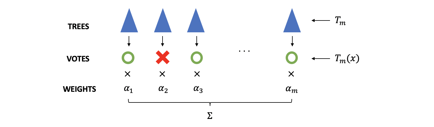
Suppose we have a binary classification tree defined as,

\hat{y} = T_m(x) \in \{-1, 1\}

$M$ trees should be,

\hat{y} = sign(\sum_{m=1}^{M}\alpha_mT_m(x))

$\alpha_m$ $M=m$ .

Screen Shot 2022-02-27 at 12.31.39 PM

Because we have,

y \in \{-1, 1\} \\ \hat{y} \in \{-1, 1\}

$y$ $\hat{y}$ are correctly classified, we have,

y\cdot \hat{y} > 0

Which is equivalent to,

y\cdot sign(\sum_{m=1}^{M}\alpha_mT_m(x)) > 0

Because the sign won't impact this inequation, then

y\cdot \sum_{m=1}^{M}\alpha_mT_m(x) > 0

$\sum_{m=1}^{M}\alpha_mT_m(x)$ $f$ , then we can write the inequation above as,

y\cdot f(x) > 0

The left term in the binary classification problem is called the margin. Therefore, we can write,

margin > 0 \Leftrightarrow y = \hat{y} \\ margin < 0 \Leftrightarrow y \neq \hat{y}

$margin = 0$ . This is equivalent to,

y\cdot f(x) = 0

Because,

y \in \{-1,1\}

we must have,

f(x) = \sum_{m=1}^{M}\alpha_mT_m(x) = 0

$f(x) = 0$ is actually defined as the decision boundary of the two classes.

(3) Recall: Log Loss For Binary Classification

$y \in \{0, 1\}$ $\hat{y} \in \{-1, 1\}$ . Recall we have discussed that the log loss for binary classification defined as,

L(y, \hat{y})=-[(y \log \hat{y}+(1-y) \log (1-\hat{y})]

$\tilde{y} = 1$ $y=1$ $\tilde{y} = -1$ $y=0$ . Then the equation above can be written as,

L(y, \hat{y})= \begin{cases} -\log \hat{y}, & \tilde{y}=1 \\<br> -\log (1-\hat{y}), & \tilde{y}=-1 \end{cases}

$\hat{y}$ $\hat{y} = sign(f(x))$ , we have, in this case,

\hat{y} = \text{sigmoid}(f(x))

Which is,

\hat{y} = \frac{1}{1+e^{-f(x)}} = (1+e^{-f(x)})^{-1}

$y=1$ ,

-\log \hat{y} = -\log (1+e^{-f(x)})^{-1} = \log (1+e^{-f(x)})

$y=0$ ,

-\log (1-\hat{y}) = -\log (1-\frac{1}{1+e^{-f(x)}}) = -\log(1+e^{f(x)})^{-1} = \log(1+e^{f(x)})

$\hat{y}$ , we have,

L(y, \hat{y})= \begin{cases} \log (1+e^{-f(x)}), & \tilde{y}=1 \\<br> \log (1+e^{f(x)}), & \tilde{y}=-1 \end{cases}

So this can also be written as,

L(y, \hat{y}) = \log (1+e^{-\tilde{y}f(x)}) \Leftrightarrow L(y, \hat{y}) = \log (1+e^{-yf(x)})

$y \in \{-1,1\}$ .

$\text{margin} = yf(x)$ for this loss function, we can have,

L(y, \hat{y})=\log {(1 + e^{-margin})}

(4) Exponential Loss and Hinge Loss

Here, we are going to introduce two more loss functions. The exponential loss function is defined as,

L(y, \hat{y})= e^{-yf(x)}= e^{-margin}

And thee Hinge loss is defined as,

L(y, \hat{y})= \max{(0, 1-yf(x))} = \max{(0, 1-margin)}

If we plot these three loss functions (i.e. log loss, exponential loss, and hinge loss) together, we can have,


17
1
import matplotlib.pyplot as plt
2
import numpy as np
3
4
x = np.linspace(-2,5,100)
5
6
y1 = np.log(1 + np.exp(-x))
7
y2 = np.exp(-x)
8
y3 = np.maximum(0, 1-x)
9
10
fig, ax = plt.subplots(1,1,figsize=(10,5))
11
ax.plot(x, y1, label="logloss")
12
ax.plot(x, y2, label="exponential")
13
ax.plot(x, y3, label="hinge")
14
ax.axhline(0, c='r', ls="--", alpha=.5)
15
16
plt.legend()
17
plt.show()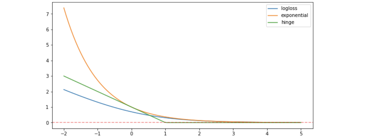

Screen Shot 2022-02-27 at 3.53.34 PM

From this plot, we can know that the loss function penalize much on the negative margins but less on the positive margins.

(5) Loss Function for AdaBoosting

$y=\{-1,1\}$ $y=\{0,1\}$ . And because exponential loss penalizes much more than the other loss functions, AdaBoosting is less robust to outliers.

For AdaBoosting, we have the overall loss function is,

Loss = \frac{1}{N}\sum_{i=1}^{N}L(y^{(i)}, \hat{y}^{(i)})= \frac{1}{N}\sum_{i=1}^{N}e^{-y^{(i)}f(x^{(i)})}

Assume our AdaBoosting model is an additive model as follows,

f(x) = \sum_{m=1}^{M}\beta_mT_m(x)

$\beta$ is the weight for each tree as our parameters. So we have the loss function as,

Loss = \frac{1}{N}\sum_{i=1}^{N}e^{-y^{(i)}\sum_{m=1}^{M}\beta_mT_m(x^{(i)})}

Or we can write the expression above in a vectorized way,

Loss = \frac{1}{N}\sum_{i=1}^{N}e^{-y^{(i)} \vec{\beta} \cdot \vec{T}(x^{(i)})}

$\mathbb{1}$ , we can write the expression above as,

Loss = \frac{1}{N} (\sum_{i=1}^{N}e^{- \vec{\beta} \cdot \vec{\mathbb{1}}_{yf>0}} + \sum_{i=1}^{N}e^{\vec{\beta} \cdot \vec{\mathbb{1}}_{yf<0}})

In order to optimize this AdaBoosting model, we have to minimize this loss function for trees and their weights,

\vec{\beta},\vec{T} = \arg \min_{\vec{\beta},\vec{T}}Loss

$T_m$ $\beta_m$ , then its loss can be written as,

Loss_m = \frac{1}{N} (\sum_{i=1}^{N}e^{- \beta_m } + \sum_{i=1}^{N}e^{\beta_m })

This is also,

Loss_m = \frac{1}{N} (N_{correct}^{(m)}e^{- \beta_m } + N_{error}^{(m)}e^{\beta_m }) = \frac{N_{correct}^{(m)}}{N} e^{- \beta_m } + \frac{N_{error}^{(m)}}{N}e^{\beta_m }

$err$ as,

err^{(m)} = \frac{N_{error}^{(m)}}{N}

Then we have,

Loss_m = (1 - err^{(m)})e^{- \beta_m } + err^{(m)} \cdot e^{\beta_m }

To minize the loss for this tree, we have,

\frac{dLoss_m}{d\beta_m} = 0

So,

-(1 - err^{(m)})e^{- \beta_m } + err^{(m)} \cdot e^{\beta_m } = 0

$\beta_m$ and then we can have,

e^{2\beta_m } = \frac{1 - err^{(m)}}{err^{(m)}}

Then,

\beta_m = \frac{1}{2}\log\frac{1 - err^{(m)}}{err^{(m)}}

$\alpha_m = 2\beta_m$ $\alpha_m$ is

\alpha_m =\log\frac{1 - err^{(m)}}{err^{(m)}}

(6) Training AdaBoosting

$i$ $w_i$ $\frac{1}{N}$ .

w_i^{(0)} = \frac{1}{N}

$m$ $i$ $T_m$ , so,

w_i \leftarrow w_i \cdot e^{-y^{(i)}\beta_mT_m(x^{(i)})}

$y^{(i)}T_m(x^{(i)}) = 1$ , this means we do not misclassify the result, and the expression above should be,

w_i \leftarrow w_i \cdot e^{-\beta_m}

$y^{(i)}T_m(x^{(i)}) = -1$ , this means we do misclassify the result, and the expression above should be,

w_i \leftarrow w_i \cdot e^{\beta_m}

$e^{-\beta_m}$ to both conditions,

w_i \leftarrow \begin{cases} w_i , & y^{(i)}T_m(x^{(i)}) = 1 \\<br> w_i \cdot e^{2\beta_m}, & y^{(i)}T_m(x^{(i)}) = -1 \end{cases}

For the fact that,

\alpha_m = 2\beta_m

We then have,

w_i \leftarrow \begin{cases} w_i , & y^{(i)}T_m(x^{(i)}) = 1 \\<br> w_i \cdot e^{\alpha_m}, & y^{(i)}T_m(x^{(i)}) = -1 \end{cases}

Where,

\alpha_m =\log\frac{1 - err^{(m)}}{err^{(m)}}

$M$ iterations should be,

f(x^{(i)}) = \sum_{m=1}^{M}\beta_mT_m(x^{(i)}) = \frac{1}{2}\sum_{m=1}^{M}\alpha_mT_m(x^{(i)})

Since we have a binary classification problem, then the hard predictions are,

F(x^{(i)}) = \text{sign} (f(x^{(i)})) = \text{sign} \sum_{m=1}^{M}\alpha_mT_m(x^{(i)})

$\frac{1}{2}$ can be ignored in this equation.

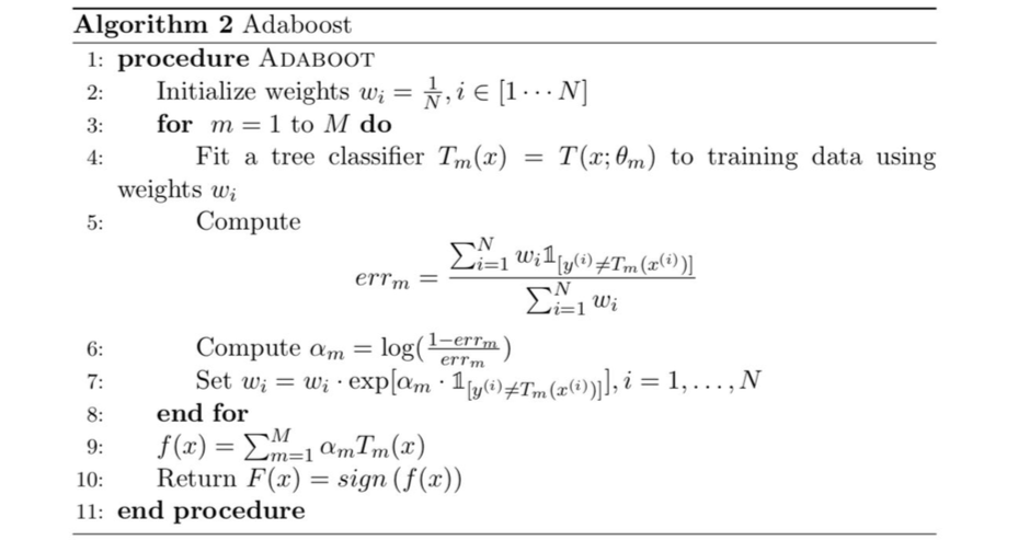
(7) Pseudo Code for AdaBoosting

Screen Shot 2022-02-28 at 2.15.54 AM

2. Gradient Boosting

(1) Idea of Gradient Boosting

$T_m(x)$ $y$ $M$ $m$ learners is,

\hat{y}_m = f_m(x^{(i)}) = f_{m-1}(x^{(i)}) + T_m(x^{(i)})

$f_m(x^{(i)})$ $y$ as their difference. We can use MSE, MAE, log loss, or some other loss functions to represent this difference.

Loss = \sum_{i=1}^{N}L(y^{(i)}, f_{m-1}(x^{(i)}) + T_m(x^{(i)}))

$f_0$ ,

f_0 = \alpha

$\alpha$ is some constant we select for this optimization.

In order to reach the optimized model, we have to minimize the loss function by steps. So in step 0, we have to solve,

\alpha = \arg\min_{\alpha} \sum_{i=1}^{N}L(y^{(i)}, \alpha)

$T_m$ that minimize the loss function,

T_m = \arg\min_{T_m} \sum_{i=1}^{N}L(y^{(i)}, f_{m-1}(x^{(i)}) + T_m(x^{(i)}))

So the idea of gradient boosting is quite similar to gradient descent because we have,

f_{m}(x^{(i)}) \leftarrow f_{m-1}(x^{(i)}) - \eta \nabla

Note that because we don't know the gradient here, we have to use a model to fit the difference between two iterations, and this difference is called the pseudo residual, which is defined as,

r_{im} = \frac {f_{m}(x^{(i)}) - f_{m-1}(x^{(i)})}{\eta} = -\nabla

Which is also,

r_{im} = -\left.\frac{\partial L}{\partial f}\right|_{f=f_{m-1}\left(x^{(i)}\right),\ y(i)}

(2) Best Initial Constant

$\alpha$ that minimize the loss function in step 0. So the best initial constant is selected based on the loss function.

$\alpha = \bar{y}$
$\alpha = \text{Median}(y)$

We can easily prove why these two constants are the best for MSE and MAE. But for the log loss, it can be tricky for calculating the best initial constant. Let's suppose we have a loss function,

L(y, f(x)) = \log (1+e^{-yf(x)})

$\alpha$ should be found by,

\alpha = \arg\min_{\alpha} \sum_{i=1}^{N}\log (1+e^{-y^{(i)}\alpha})

Then,

\frac{d\sum_{i=1}^{N}\log (1+e^{-y^{(i)}\alpha})}{d\alpha} = -\sum_{i=1}^{N} \frac{1}{1+e^{-y^{(i)} \alpha}} y^{(i)} e^{-y^{(i)} \alpha}=0

So,

\sum_{i=1}^{N} \frac{y^{(i)}}{1+e^{y^{(i)} \alpha}}=0

$y^{(i)} \in \{1, -1\}$ $N^+$ $y^{(i)}= 1$ $N^-$ $y^{(i)}= -1$ . So we have,

N = N^+ + N^-

Therefore,

\sum_{i=1}^{N} \frac{y^{(i)}}{1+e^{y^{(i)} \alpha}} = \frac{N^+}{1+e^{ \alpha}} - \frac{N^-}{1+e^{ -\alpha}}=0

So,

\frac{N^+}{1+e^{ \alpha}} = \frac{N^-}{1+e^{ -\alpha}}

Then,

\frac{N^+}{1+e^{ \alpha}} = \frac{N^-e^{ \alpha}}{1+e^{ \alpha}}

So,

N^+ = N^-e^{ \alpha}

And,

\alpha = \log \frac{N^+}{N^-}

Note that we have,

\frac{1+\bar{y}}{1-\bar{y}}=\frac{1+\frac{N^{+}-N^{-}}{N}}{1-\frac{N^{+}-N^{-}}{N}}=\frac{N+N^{+}-N^{-}}{N-N^{+}+N^{-}} =\frac{N^+}{N^-}

$\alpha$ is also,

\alpha = \log \frac{1+\bar{y}}{1-\bar{y}}

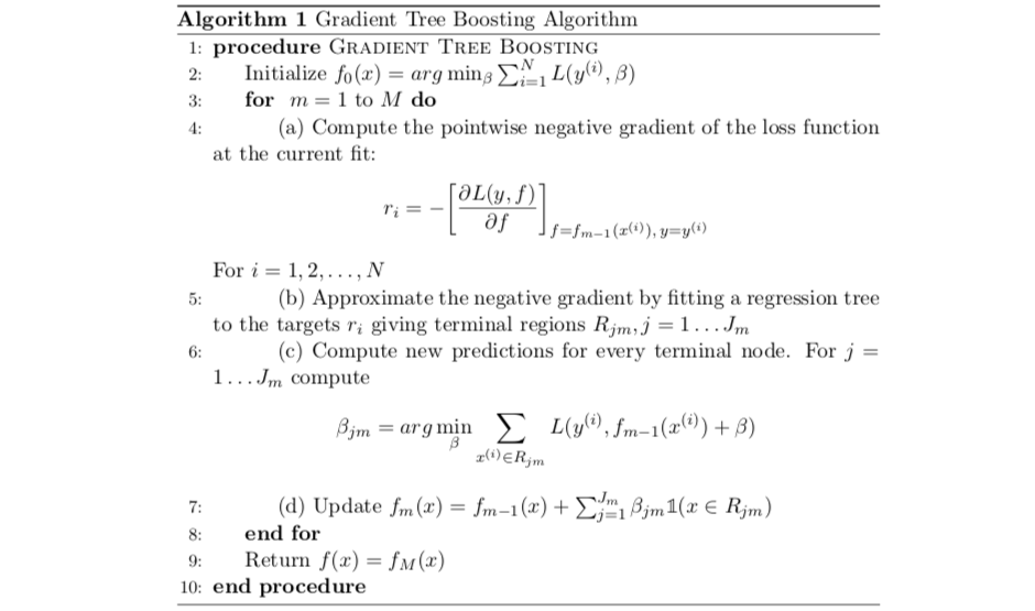
(3) General Tree Gradient Boosting

As we have already defined the pseudo residual is,

r_{im} = -\left.\frac{\partial L}{\partial f}\right|_{f=f_{m-1}\left(x^{(i)}\right),\ y(i)}

$x_i$ $r_i$ ,

T_m(x_i) \sim r_i

$R_{jm}$ $T_m$ $x_i \in R_{jm}$ , make new predictions by minizing the loss fuction,

\beta_{j m}=\arg \min _{\beta} \sum_{x^{(i)} \in R_{j m}} L\left(y^{(i)}, f_{m-1}\left(x^{(i)}\right)+\beta\right)

$f_m$ with the new predictions,

f_{m}(x)=f_{m-1}(x)+\sum_{j=1}^{J_{m}} \beta_{j m} \mathbb{1}\left(x \in R_{j m}\right)

(4) Pseudo Residual For Logloss

Since we have the definition of pseudo residual as,

r_{im} = -\left.\frac{\partial L}{\partial f}\right|_{f=f_{m-1}\left(x^{(i)}\right),\ y^{(i)}}

And the logloss is defined by,

L(y, f)=\log {(1 + e^{-yf})}

Then,

r_{im} = -\left.\frac{\partial \log {(1 + e^{-yf})}}{\partial f}\right|_{f=f_{m-1}\left(x^{(i)}\right),\ y^{(i)}}

This is also,

r_{im} = -\left.\frac{-y \cdot e^{-yf}}{\log {(1 + e^{-yf})}}\right|_{f=f_{m-1}\left(x^{(i)}\right),\ y^{(i)}}

So,

r_{im} = -\left.\frac{-y}{\log {(1 + e^{yf})}}\right|_{f=f_{m-1}\left(x^{(i)}\right),\ y^{(i)}} = \frac{y^{(i)}}{\log {(1 + e^{y^{(i)}f_{m-1}(x^{(i)})})}}

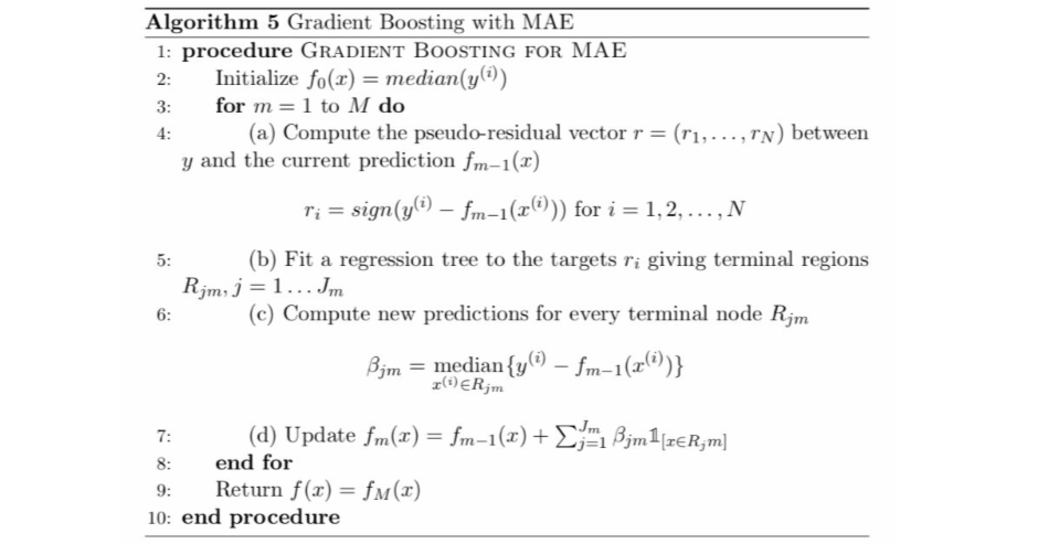
(5) Pseudo Residual For MSE and MAE

For MSE, the pseudo residual is quite simple with,

MSE = (y-f)^2

Then,

r_{im} = -\left.\frac{\partial (y-f)^2}{\partial f}\right|_{f=f_{m-1}\left(x^{(i)}\right),\ y^{(i)}} = -2(y^{(i)}-f_{m-1}(x^{(i)}))

For MAE, the loss function is,

MAE = |y - f|

Then,

r_{im} = -\left.\frac{\partial |y - f|}{\partial f}\right|_{f=f_{m-1}\left(x^{(i)}\right),\ y^{(i)}}

This is to say we have,

r_{im} = \begin{cases} -\left.\frac{\partial (y - f)}{\partial f}\right|_{f=f_{m-1}\left(x^{(i)}\right),\ y^{(i)}} , & y-f\geq0 \\<br> -\left.\frac{\partial (f-y)}{\partial f}\right|_{f=f_{m-1}\left(x^{(i)}\right),\ y^{(i)}}, & y-f<0 \end{cases}

Then,

r_{im} = \begin{cases} 1 , & y-f\geq0 \\<br> -1 , & y-f<0 \end{cases}

So that we can conclude that, for MAE, the pseudo result can be written as,

r_{im} = sign(y^{(i)}-f_{m-1}(x^{(i)}))

(6) Pseudo Residual for Exponential Loss

We can continue to derive the pseudo residual for exponential loss. The loss function is defined as,

L(y, f)=e^{-yf}

So for the definition of pseudo residual,

r_{im} = -\left.\frac{\partial e^{-yf}}{\partial f}\right|_{f=f_{m-1}\left(x^{(i)}\right),\ y^{(i)}} = y^{(i)} \cdot e^{-y^{(i)}f_{m-1}\left(x^{(i)}\right)}

(7) Pseudo Residual for Hinge Loss

The last pseudo residual we are going to have a look at is with the hinge loss. Suppose the loss function is,

L(y, f)= \max{(0, 1-yf)}

It can also be written as,

L(y, f)= \begin{cases}<br> 0, & yf \geq 1\\<br> 1-yf, & yf < 1<br> \end{cases}

$L$ $f$ is,

r_{im} = \begin{cases}<br> 0, & yf \geq 1\\<br> -\left.\frac{\partial (1-yf)}{\partial f}\right|_{f=f_{m-1}\left(x^{(i)}\right),\ y^{(i)}}, & yf < 1<br> \end{cases}

So we have,

r_{im} = \begin{cases}<br> 0, & yf \geq 1\\<br> y^{(i)}, & yf < 1<br> \end{cases}

(8) Best Constant Per Region for Logloss

After getting the pseudo residual and fitting the model , then, the next step is to find the optimal constant per region. For logloss, that is,

\begin{aligned}<br>\beta_{j} &=\arg \min _{\beta} \sum_{x^{(i)} \in R_{j}} L\left(y^{(i)}, f_{m-1}\left(x^{(i)}\right)+\beta\right) \\<br>&=\arg \min _{\beta} \sum_{x^{(i)} \in R_{j}} \log \left(1+e^{-y^{(i)}\left[f_{m-1}\left(x^{(i)}\right)+\beta\right]}\right)<br>\end{aligned}

Then the derivative is,

G(\beta) = \frac {\partial \sum_{x^{(i)} \in R_{j}} \log \left(1+e^{-y^{(i)}\left[f_{m-1}\left(x^{(i)}\right)+\beta\right]}\right)}{\partial \beta} = -\sum_{x^{(i)} \in R_{j}} \frac{y^{(i)}}{1+e^{y^{(i)}\left[f_{m-1}\left(x^{(i)}\right)+\beta\right]}}

$G(\beta)=0$ $\beta$

\beta = -\frac{G(0)}{G'(0)}

$G'(\beta)$ is ,

G^{\prime}(\beta)=\sum_{x^{(i)} \in R_{j}} \frac{\left(y^{(i)}\right)^{2} e^{y^{(i)}\left[f_{m-1}\left(x^{(i)}\right)+\beta\right]}}{(1+e^{\left.y^{(i)}\left[f_{m-1}(x^{(i)}\right)+\beta\right]})^{2}}

Note that,

-G(0)=\sum_{x^{(i)} \in R_{j}} \frac{y^{(i)}}{1+e^{y^{(i)}\left[f_{m-1}\left(x^{(i)}\right)\right]}}=\sum_{x^{(i)} \in R_{j}} r_{i}

And,

\left|r_{i}\right|=\frac{1}{1+e^{y^{(i)} \cdot f_{m-1}\left(x^{(i)}\right)}}

So,

1-\left|r_{i}\right|=\frac{e^{y^{(i)} \cdot f_{m-1}\left(x^{(i)}\right)}}{1+e^{y^{(i)} \cdot f_{m-1}\left(x^{(i)}\right)}}

Therefore,

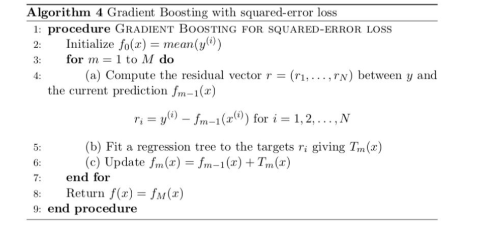
\beta_{j}=\frac{\sum_{x^{(i)} \in R_{j}} r_{i}}{\sum_{x^{(i)} \in R_{j}}\left|r_{i}\right|\left(1-\left|r_{i}\right|\right)}

(9) General Pseudo Code for Gradient Tree Boosting

Screen Shot 2022-02-28 at 2.09.37 AM

(10) Pseudo Code for Gradient Tree Boosting with MAE Loss

Screen Shot 2022-02-28 at 2.12.46 AM

(11) Pseudo Code for Gradient Tree Boosting with MSE Loss

Screen Shot 2022-02-28 at 2.14.20 AM