Data Structure and Algorithm 1 | Algorithm Analysis Theory

0. Environment Installation

• Download the jar file algs4.jar to root directory

xxxxxxxxxx
1
1
$ sudo curl -O "https://algs4.cs.princeton.edu/code/algs4.jar"

• Install the command line tools

xxxxxxxxxx
3
1
$ sudo curl -O "https://algs4.cs.princeton.edu/linux/{javac,java}-{algs4,cos226,coursera}"
2
$ sudo chmod 755 {javac,java}-{algs4,cos226,coursera}
3
$ sudo mv {javac,java}-{algs4,cos226,coursera} /usr/local/bin

• Download and install the latest version IntelliJ IDEA community version

1. Basic Concepts

As soon as an Analytic Engine exists, it will necessarily guide the future course of the science. Whenever any result is sought by its aid, the question will arise — By what course of calculation can these results be arrived at by the machine in the shortest time?

— Charles Babbage (1864)

In Java, we can time the running time of an algorithm by Stopwatch class, which is a part of the stdlib.jar. We should use Stopwatch() for creating a new stopwatch and then call elapsedTime() to get the time in seconds since the Stopwatch is created.

xxxxxxxxxx
10
1
public class Stopwatch {
2
    private final long start;
3
    public Stopwatch() {
4
        start = System.currentTimeMillis();
5
    }
6
    public double elapsedTime() {
7
        long now = System.currentTimeMillis();
8
        return (now - start) / 1000.0;
9
    }
10
}

(1) Scientific Method

In the 1970s, Donald Knuth introduces the scientific method for understanding computing performance. Nowadays, the scientific method is explained in the following steps,

• Observe some features of the natural world.
• Hypothesize a model that is consistent with the observations.
• Predict events using the hypothesis.
• Verify the predictions by making further observations.
• Validate by repeating until the hypothesis and observations agree

There are two principles for the scientific method,

• Experiments must be reproducible
• Hypotheses must be falsifiable

2. Examples of Successful Algorithms

(1) Discrete Fourier Transform (DFT) Problem

Break down waveform of N samples into periodic components. The applications are on DVDs, JPEG files, MRI, astrophysics, etc.

• Brute Force: N² steps
• Fast Fourier Transform: NlogN steps (called linearithmic)

(2) N-Body Simulation Problem

Simulate gravitational interactions among N bodies.

• Brute Force: N² steps
• Barnes-Hut algorithm: NlogN steps

(3) Three Sum Problem

Given N distinct integers, how many triples sum to exactly zero?

For example,

xxxxxxxxxx
1
1
1 2 -1 0 -2

The answer should be,

xxxxxxxxxx
3
1
2
2
1 + -1 + 0 = 0
3
2 + -2 + 0 = 0

• Brute Force: Grid-search (n³ complexity)

xxxxxxxxxx
5
1
for (int i = 0; i < n; i++) 
2
    for (int j = i + 1; j < n; j++) 
3
        for (int k = j + 1; k < n; k++) 
4
            if (a[i] + a[j] + a[k] == 0) 
5
               count++;

The Grid-search program should be,

​x
1
import edu.princeton.cs.algs4.StdIn;
2
import edu.princeton.cs.algs4.StdOut;
3
import edu.princeton.cs.algs4.In;
4
​
5
public class ThreeSum {
6
​
7
    private ThreeSum() {
8
    }
9
​
10
    public static int count(int[] a) {
11
        int n = a.length;
12
        int count = 0;
13
        for (int i = 0; i < n; i++) {
14
            for (int j = i + 1; j < n; j++) {
15
                for (int k = j + 1; k < n; k++) {
16
                    if (a[i] + a[j] + a[k] == 0) {
17
                        count++;
18
                    }
19
                }
20
            }
21
        }
22
        return count;
23
    }
24
​
25
    public static void main(String[] args) {
26
        In in = new In(args[0]);
27
        int[] a = in.readAllInts();
28
​
29
        Stopwatch timer = new Stopwatch();
30
        int count = count(a);
31
        StdOut.println("elapsed time = " + timer.elapsedTime());
32
        StdOut.println(count);
33
    }
34
}

We can download the testing files of 1Kint.txt, 2Kint.txt , 4Kint.txt , and 8Kint.txt (nKint means we have n thousand integers in that file) from these links. And then we are able to test these files by,

xxxxxxxxxx
4
1
$ java-algs4 ThreeSum 1Kints.txt
2
$ java-algs4 ThreeSum 2Kints.txt
3
$ java-algs4 ThreeSum 4Kints.txt
4
$ java-algs4 ThreeSum 8Kints.txt

The results are,

xxxxxxxxxx
5
1
Name                Time                Result         
2
1Kints.txt          0.296               70
3
2Kints.txt          2.679               528
4
4Kints.txt          22.225              4039
5
8Kints.txt          170.302             32074

If we plot this result with the standard plot and the log-log plot, we will have the following relationships,

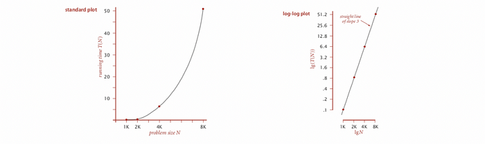
This is because we have,

xxxxxxxxxx
1
1
T(N) = a * N^b

So,

xxxxxxxxxx
1
1
log(T(N)) = blog(N) + c

where,

xxxxxxxxxx
1
1
a = exp(c)

Because we have a slope in this plot of about 3, then we can say,

xxxxxxxxxx
1
1
b = 3

And the order of growth of the running time is about,

xxxxxxxxxx
1
1
N^3

• Quick ThreeSum: Applying the binary search algorithm as the last loop. We will leave the discussion of binarySearch later in this series.

xxxxxxxxxx
6
1
for (int i = 0; i < N; i++) {
2
    for (int j = i+1; j < N; j++) {
3
        int k = Arrays.binarySearch(a, -(a[i] + a[j]));
4
        if (k > j) cnt++;
5
    }
6
}

xxxxxxxxxx
30
1
import java.util.Arrays;
2
import edu.princeton.cs.algs4.StdIn;
3
import edu.princeton.cs.algs4.StdOut;
4
import edu.princeton.cs.algs4.In;
5
​
6
public class ThreeSumFast {
7
​
8
    public static int count(int[] a) {
9
        int N = a.length;
10
        Arrays.sort(a);
11
        int cnt = 0;
12
        for (int i = 0; i < N; i++) {
13
            for (int j = i+1; j < N; j++) {
14
                int k = Arrays.binarySearch(a, -(a[i] + a[j]));
15
                if (k > j) cnt++;
16
            }
17
        }
18
        return cnt;
19
    }
20
​
21
    public static void main(String[] args)  {
22
        In in = new In(args[0]);
23
        int[] a = in.readAllInts();
24
​
25
        Stopwatch timer = new Stopwatch();
26
        int count = count(a);
27
        StdOut.println("elapsed time = " + timer.elapsedTime());
28
        StdOut.println(count);
29
    }
30
}

Again, we can simulate the time by,

xxxxxxxxxx
4
1
$ java-algs4 ThreeSumFast 1Kints.txt
2
$ java-algs4 ThreeSumFast 2Kints.txt
3
$ java-algs4 ThreeSumFast 4Kints.txt
4
$ java-algs4 ThreeSumFast 8Kints.txt

The results are,

xxxxxxxxxx
5
1
Name                Time                Result         
2
1Kints.txt          0.019               70
3
2Kints.txt          0.090               528
4
4Kints.txt          0.257               4039
5
8Kints.txt          1.504               32074

Here, we can spot a big improvement in the time complexity.

3. Algorithm Theory

(1) The Definition of Algorithm Analysis

The algorithm analysis theory is invented in the book The Art Of Computer Programming by Donald Knuth. It explains the mathematical models for calculating the total running time of a computer program, which should physically be the sum of cost times frequency for all operations.

• Cost depends on machine and compiler
• Frequency depends on algorithm and input data

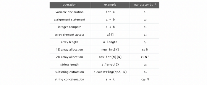
(2) Cost of Basic Operations

(3) Brute-Force TwoSum Cost Example

Now, let’s analyze the cost of a TwoSum program. In this program, we have,

xxxxxxxxxx
5
1
int count = 0; 
2
for (int i = 0; i < N; i++) 
3
    for (int j = i+1; j < N; j++) 
4
        if (a[i] + a[j] == 0) 
5
           count++;

Then, the frequency for each operation should be,

xxxxxxxxxx
19
1
// 1 time int count; 1 time int i; N times int j;
2
variable declaration                                    N + 2
3
​
4
// 1 time count = 0; 1 time i = 0; N times j = i + 1;
5
assignment statement                                    N + 2
6
​
7
// N+1 times i < N; N(N+1)/2 times j < N
8
less than compare                N+1 + N(N+1)/2 =    (N+1)(N+2)/2
9
​
10
// (N-1) + ... + 2 + 1 + 0 times x == 0;
11
equal to compare                                       N(N-1)/2
12
​
13
// N(N-1)/2 times a[i]; N(N-1)/2 times a[j];
14
array access                                            N(N-1)
15
​
16
// at worst: N(N-1)/2 times count++; N(N-1)/2 times a[i] + a[j];
17
// at best: no count++; N(N-1)/2 times a[i] + a[j];
18
// ignore i++ and j++;
19
increment                                         N(N-1)/2 to N(N-1)

The cost model is to use some basic operations as a proxy for running time and here we can simply choose array access with the cost model N(N-1).

(4) Tilde Notation

The tilde notation ~ is used when we are able to ignore lower order terms, so technically,

When,

Then, for the Brute-Force TwoSum problem, the can be cost model with N inputs can be simplified to N².

xxxxxxxxxx
1
1
N(N-1) ~ N²

(5) Big-Oh Notation

The most commonly used notation in algorithm analysis is the big-oh notation O. It also has two friends, big-theta Θ and big-omega Ω.

• Big-Theta: Θ(f(N)) is a notation that stands for a polynomial with the highest order term ~ f(N). For example,

xxxxxxxxxx
1
1
N² + 2N + 1  ~  Θ(N²)

• Big-Oh (upper bound): O(f(N)) is a notation that stands for a polynomial with the highest order term ~ f(N) or smaller. For example,

xxxxxxxxxx
2
1
N² + 2N + 1  ~  O(N²)
2
2N + 1       ~  O(N²)

• Big-Omega (lower bound): Ω(f(N)) is a notation that stands for a polynomial with the highest order term ~ f(N) or larger. For example,

xxxxxxxxxx
2
1
N² + 2N + 1  ~  Ω(N²)
2
N³ + 2N + 1  ~  Ω(N²)

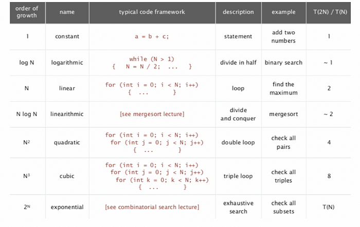
(6) Common Order of Growth Classifications

(7) Problem Sizes Per Minute for Different Order of Growth in the 2000s

xxxxxxxxxx
9
1
growth-rate                       Problem Size
2
1                                          any
3
logN                                       any
4
N                                1,000,000,000
5
NlogN                              100,000,000
6
N²                                      10,000
7
N²logN                                  10,000
8
N³                                       1,000
9
2^N                                         30

(8) Memory Cost for Common Data Type

13
1
boolean                 1
2
byte                    1
3
char                    2
4
int                     4
5
float                   4
6
long                    8
7
double                  8
8
char[]            2N + 24
9
int[]             4N + 24
10
double[]          8N + 24
11
char[][]          ~ 2 M N
12
int[][]           ~ 4 M N
13
double[][]        ~ 8 M N