High-Performance Computer Architecture 4 | Metrics and Evaluation of Performance, Iron Law…
High-Performance Computer Architecture 4 | Metrics and Evaluation of Performance, Iron Law, Amdahl’s Law, and Lhadma’s Law

- Performance Measurements
(1) The Definition of Latency and Throughput
Usually, we say performance, we mean the “processor speed”. But even then, there are really two aspects of performance that are not necessarily identical. One is called latency, the other is called throughput.
- Latency: How long does a thing take from when we start something until it’s done.
- Throughput: How many things can we do per second.
We will see why they are not identical.
(2) The Relationship Between Latency and Throughput
Some may think that the value of the throughput is actually 1 over latency, which is,

However, this is NOT right. Let’s think about an example. Suppose we have a task that has a latency of 4 seconds. Then by the expression above, we may calculate that,
throughput = 1/4 = 0.25
This is not right because, in reality, the tasks are always divided into many steps and we don’t have to wait for the last task if we want to start a new task. This means that the real throughput can be much higher than 0.25 and 0.25 is a just extreme case of the throughput.
Let’s see now see another example. Suppose we have 2 servers and for processing online orders and each order request is assigned to one of the two servers. Each server takes 1 ms to process the order and it can not do anything else while processing an order. In this case, because each task needs 1ms to be processed, so by definition, the latency should be 1 ms . However, the throughput is not 1,000 orders per second because we have two servers working at the same time. Thus, the throughput should be 2,000 orders per second.
(3) Comparing Performance By Speedup
Let’s now see how do we compare the performance through the latency and throughput. If we say “Computer X is N times faster than Y” or the speedup of X and Y is N, then the speedup N can be computed by,

If we use throughput as the measure of the speed, then,

However, if we use latency as the measure of the speed, because latency is negatively related to each other, then,

(4) Speedup Interpretation
When the value of speedup is larger than 1, then,
- Improved performance
- Shorter execution time
- Higher throughput
When the value of speedup is smaller than 1, then,
- Worse performance
- Longer execution time
- Lower throughput
(5) The Definition of Benchmark Workloads
Now, let’s think about how to measure performance. We have seen that we can express performance by 1 over execution time. But there’s a question remaining that what is the workload for this execution time? A simple idea is to use the actual user workload. However, this idea is useless in practice for three main reasons,
- too many programs
- not representative of other users
- privacy concerns
Instead, we use the benchmark workloads for measuring the performance. The benchmark workload is a series of programs and input data that users and companies have agreed upon will be used for performance measures.
Usually, we don’t have only one benchmark program. A benchmark suite contains multiple programs along with the input data and each of these programs is usually chosen to be representative of some type of applications.
(6) Types of Benchmarks
- Real applications benchmarks: are the most representative benchmark. But they are also the most difficult ones to set up on a new machine (for example, we may need to configure the environment, install the drives and apps, etc.).
- Kernel benchmarks: We can find the most time-consuming part of an application (usually a loop). Thus, we don’t have to install all the drives or relative stuff for the real application. But a reasonably sized kernel is still too difficult for a prototyped machine or an early staged computer (sometimes we even don’t have a compiler). When we actually build a machine for the first time as a prototype, we can use this kind of benchmark.
- Synthetic benchmarks: These benchmarks are usually designed to behave similarly to some type of kernel but they are much simpler to compile. These benchmarks are usually good for design studies, but they are not a good idea to report to others, especially our customers.
- Peak performance benchmarks: The above methods are to compare machines based on some actual codes but there’s also a measure of the peak performance that tells us the performance. In theory, peak performance tells us how many instructions per second should this machine be able to execute. However, this measurement is only used for marketing because it can deviate from the actual performance of a machine. peak performance
(7) Benchmark Standards
Usually, there are standard organizations that put together benchmark suites for comparing machines. A standard organization takes inputs from manufacturers, user groups, and experts in academia to produce a standard benchmark suite along with instructions on how to produce representative measurements.
- TPC benchmark: standard benchmark used for database, web servers, data mining, and other transaction processing
- EEMBC benchmark: standard benchmark used for embedded processing such as cars, video players, printers, mobile phones, etc.
- SPEC benchmark: standard benchmark typically used to evaluate engineering workstations and also our processors because these benchmarks are not very I/O intensive. This kind of benchmark includes several applications (i.e. GCC — software development workloads like compiler, BEWAVES & LBM — Floyd dynamic workloads, PERL — string processing applications, CACTUS ADM — physics simulation, XALANC BMK — for XML, CALCULIX & DEALL—for differential equations, BZIP — for compression application, GO & SJENG — for game AI applications).
(8) Performance Summarizing Methods
- Average execution time: calculate the average time for each execution and then calculate the speedup. We can not simply average the values of the speedups. This is the commonest method we normally use for summarizing performance
- Geometric mean: if we want to calculate the mean value by the speedups, we have to use the geometric mean. We are going to use the geometric mean only if we don’t know the actual time for each application. The geometric mean is defined by,

Let’s see an example. Where AVG represents average execution time and GEO means for geometric mean,
           COMP_X    COMP_Y     SPEEDUP
APP A        9        18          2
APP B       10         7          0.7
APP C        5        11          2.2
AVG          8        12          1.5
GEO          7.66     11.15       1.46
2. Iron Law of Performance
(1) CPU Time
In this series, we are going to focus mainly on the processor. When we say processor, we are always meaning the CPU (central processing unit). The CPU time or the processor time is defined as the time for a processor to run a program.
(2) Iron Law of Performance
Actually, the CPU time can be calculated by,

This can be proved by the following expression,

The three components of the CPU time allow us to think about different aspects of computer architecture. This is called the Iron Law of performance. We can also write this expression to,

where,
- IC means instructions count
- CPI means cycles per instruction
- CCT means clock cycle time (which is also the reciprocal of the cycle clock)
(3) Components of the CPU Time And Computer Architecture
- # of instructions per program: generally affected by the algorithm we use and the compiler we use. Also, the instruction set can impact how many instructions we need for a program
- # of cycles per instruction: affected by the instruction set (a simple set will reduce the cycles to do) and the processor design
- clock cycle time: affected by the processor design, the circuit design, and the transistor physics
(4) Iron Law for Unequal Instruction Times
The iron law of performance can be easily applied to the instructions that have constant cycles, but how can we apply this law to the unequal instruction times. This is a simple mathematic problem and the final processor time can be calculated by,

3. Amdahl’s Law
(1) Definition of the Amdahl’s Law
Another law we may use a lot is called the Amdahl’s Law, especially when we are about to speed up only part of the program or only some instructions. Basically, when are have a speed-up task but it doesn’t apply to the entire program and we want to know what is the overall speed up on the entire program.
The fraction enhanced is defined as the percentage of the original execution TIME (not instructions count or something else) that is affected by our enhancement and this value is denoted as FRAC_enh.
By Amdahl’s Law, the overall speedup can be calculated by,
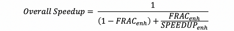
(2) Amdahl’s Law Implications
So what does Amdahl’s law implies? Let’s think about two different enhancements. For enhancement #1, we enhance a speedup of 20 on 10% of the time. For enhancement #2, we enhance a speedup of 1.6 on 80% of the time. By Amdahl’s law, the overall speedup for enhancement #1 is 1.105 and the overall speedup for enhancement #2 is 1.43 .
This implies that if we put significant effort to speed up something that is a small part of the execution time, you will still not get a very large improvement. In contrast, if you are impacting a large part of the execution time and even if there’s only a small reasonably small speedup, you will still result in a large overall speedup.
4. Lhadma’s Law
This is jokingly called Lhadma’s law because of Amdahl’s law. We have known that Amdahl’s law implies that we have to speed up the most common cases in order to have a significant impact on the overall speedup, while Lhadma’s law tells us that we don’t want to mess up with the uncommon cases too badly.
Let’s see an example. Suppose we would like to have a speedup of 2 on 90% of the execution time and another speedup of 0.1 on the rest of the execution time. The overall speedup can be calculated by,

And this result proves Lhadma’s law.
5. Diminishing Returns
The diminishing returns is another rule that tells us not to go overboard improving the same thing because the thing that has been already improved are now a smaller percentage of the new execution time and we need to reassess what is now the dominate part. In other words, this also mentions that we have to reconsider what is now the enhancement percentage after each speeding up.