High-Performance Computer Architecture 5 | Set Up the Virtual Machine and Simulator, Report…
High-Performance Computer Architecture 5 | Set Up the Virtual Machine and Simulator, and Report Interpretation

- Set Up the Virtual Machine
(1) VirtualBox Installation
In this section, we would like to set up the experiment environment by the virtual machine. To continue, let’s download and install the Oracle VM VirtualBox 6.1 (if there’s a new version, download the new one) from this link (for Mac OS). Then, this should be installed as the VirtualBox application.

(2) Download the Virtual Machine
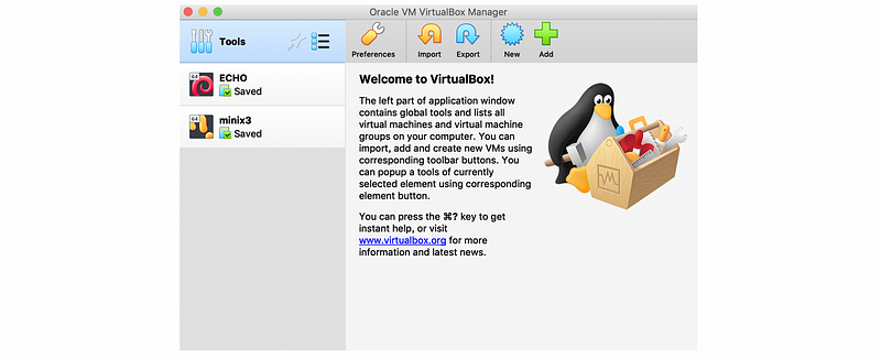
A virtual machine is an emulation of a computer system and we can import machines by the OVA file. First, let’s download the project virtual machine from google drive (about 1.6 GB). And then, we should open the VM and from here you can find the import button at the top,
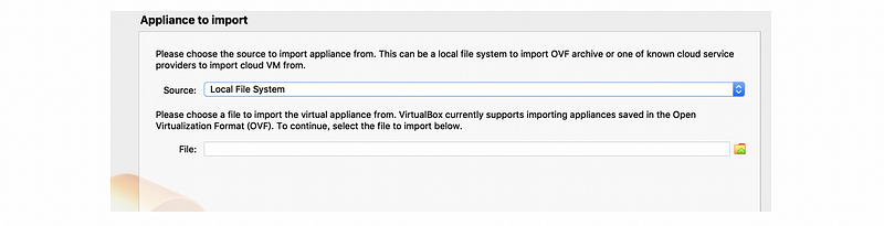
After click on the import button, we can then choose an OVA file to import. In this case, our file is called CS6290 Project VM.ova . Then click on “Continue” to import the file,
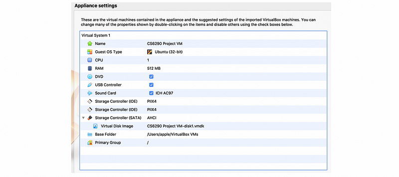
Then, a list of settings of this virtual machine is now displayed for us. We can find out that the OS for our virtual machine is Ubuntu (32-bit) with 512 MB RAM. Click on “Import” to import this virtual machine,
Now, we are going to have this virtual machine in the VirtualBox,
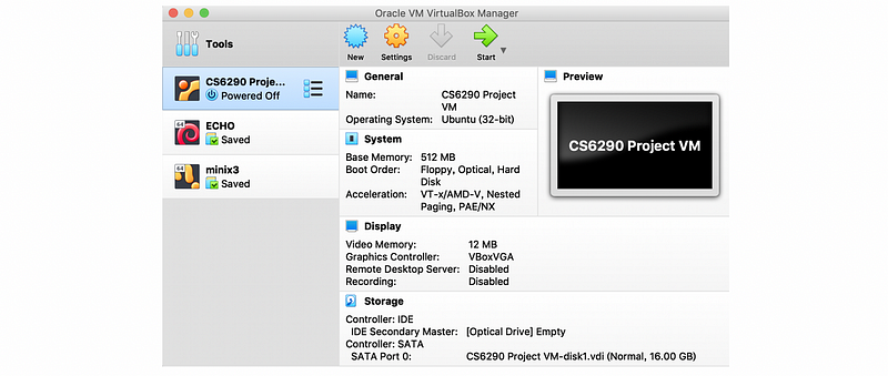
And we can click on the button “Start” at the top to start this machine.
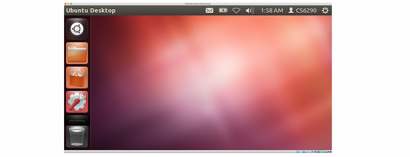
Note that you may want to change the display settings from the preference to 1920 * 1080 . To continue, let’s first shut down the machine.
A shared folder can be useful for backups and shared files. We can set up a shared folder with the following steps,
1) Create a directory on the host machine.
2) Shutdown the VM if it’s running.
3) In the settings for the VM, go to the “Shared Folders” tab.
4) Right-click “Machine Folders” then select “Add Shared Folder”.
5) Fill in this information:
- Folder Path = {path to shared folder}
- Auto-mount = checked
6) Reboot the VM.
7) Find the shared folder under “/media” named with sf_….
2. Simulator Set-up
The simulator in the sesc directory within our home directory, and we first need to build it.
$ cd ~/sesc
$ make
Then,
$ cd apps/Splash2/lu
Then,
$ make
In the same directory, run
$ ~/sesc/sesc.opt -fn64.rpt -c ~/sesc/confs/cmp4-noc.conf -olu.out -elu.err lu.mipseb -n64 -p1
Where,
- the
-foption tells the simulator to create a report file that ends with a dot and the specified string. The name of the report file issesc_followed by the name of the executable for the simulated application (lu.mipsebin this case), followed by a dot.and the stringn64.rptwe specify here. -coption tells the simulator which configuration file to use. In this case, we are using the file named~/sesc/confs/cmp4-noc.conf.- The
-oand-eoptions tell it to save the standard and error output of the application intolu.outandlu.errfiles, respectively. - The
-n64parameter tells the LU application (which does LU decomposition of a matrix) to work on a64 * 64matrix. - The
-p1parameter tells the application to use only one core.
Check there are no errors,
$ cat lu.err
And the output should end with Total time without initialization: 0
$ cat lu.out
Note that there is also a report named sesc_lu.mipseb.n64.rpt that we can read the information about the command line we used, a copy of the hardware configuration we used, and then lots of information about the simulated execution we have just completed. To show this report, we can run,
$ ~/sesc/scripts/report.pl sesc_lu.mipseb.n64.rpt
3. Report Interpretation
In this part, we are going to meet some concepts like branch . If you don’t understand these so far, don’t worry and we will explain more about these in the following sections.
The printout of the report script gives us the command line that was used, then tells us how fast the simulation was going by Exe Speed, how much real-time elapsed while the simulator was running Exe Time, and how much simulated time on the simulated machine it took to run the benchmark Sim Time. For example,
Exe Speed       Exe MHz         Exe Time         Sim Time (1000MHz)
---- KIPS       ---- MHz        ---- secs            ---- msec
The printout of the report script also tells us how accurate the simulated processor’s branch predictor was overall (the number under Total). The next two numbers are in parenthesis under the RAS label, and they report the accuracy of the return address stack RAS and what percentage of branches have actually used the RAS.
Next, under the BPred label, we have the accuracy for branches that didn’t use the RAS (i.e. they used the direction predictor and possibly the BTB and/or the BTAC), and then we have statistics for the BTB and BTAC, which are less interesting for now.
Total           RAS          BPred          BTB           BTAC
---- % ( ---- % of ---- %)   ---- % ( ---- % of ---- %)   ---- %
Next, the report tells us how many dynamic instructions were completed nInst (Instructions Count) and the breakdown of these instructions, i.e. the percentage of nInst that comes from control flow instructions like branches, jumps, calls, returns, etc. (the number under the BJ label), from loads Load, from stores Store, from integer ALU INT, and from floating-point ALU operations FP. The rest of that line (LD Forward and beyond) is less interesting for now. For example,
nInst BJ Load Store INT FP : LD Forward , Replay : Worst Unit (clk)
Next, the report tells us the overall IPC (Instructions per second) achieved by the simulated processor on this application, how many cycles the processor spent trying to execute instructions, and what those cycles were spent on. This last part is broken down into issuing useful instructions Busy, waiting for a load queue entry LDQ to become free, then the same for store queue STQ, reservation stations IWin, ROB entries, and physical registers (Regs, the simulator uses a Pentium 4-like separate physical register file for register renaming).
Some of the cycles are wasted on TLB misses TLB, on issuing wrong-path instructions due to branch mispredictions MisBr, and some other more obscure reasons (Ports, maxBr, Br4Clk, Other). Note that each of these “how the cycles were spent” items is a percentage although they do not have the percentage sign.
IPC Cycles Busy LDQ STQ IWin ROB Regs Ports TLB maxBr MisBr Br4Clk Other
Also note that the simulator models a multiple-issue processor, so the breakdown of where the cycles went is actually attributing partial cycles when needed. For example, in a four-issue processor, we may have a cycle where one useful instruction is issued and then the processor could not issue another one because the LDW became full. In this cycle, 0.25 cycles would be counted as Busy and 0.75 cycles toward LDQ.