High-Performance Computer Architecture 6 | Basis of Pipelining, Pipeline Dependencies and Hazards…
High-Performance Computer Architecture 6 | Basis of Pipelining, Pipeline Dependencies and Hazards, and Pipeline Stages

- Basis of Pipelining
(1) Introduction to Pipelining
There are several key concepts that are used in many ways in computer architecture. One of these concepts is called pipelining and it is used in several ways in pretty much every computer nowadays.
Pipelining is crucial to improving performance in processors; it increases throughput and reduces cycle time. The downside of pipelines is the increase in hazards for both controls and data.
(2) The Real Oil Pipeline
So how do pipelining works? Let’s think about the following metaphor. Suppose we want to transport oil between a filling station and an oil production plant and we have two methods to do that. One is to transport the oil through a tank truck, while the other one is through an oil pipeline.
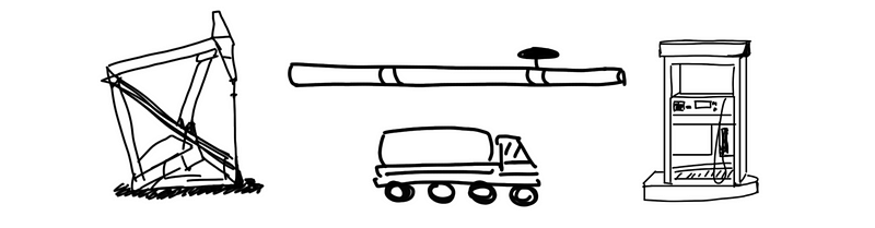
As we have already known that the oil needs three days to flow from one side to the other side, and the truck also needs three days to drive from the plant to the station. Let’s say the throughput of the pipeline can fill the trunk in 1 hour and suppose that this is a new pipeline (not filled with oil by the starting time). If we want to transport 2 trucks of oil and we have only 1 tank truck, which method is more time-efficient? Note that the time for a truck to fill in the station can be ignored.
The answer is by pipeline! For the first truck of oil, the pipeline needs 3 days (from one side to another) plus 1 hour (fill in the station) and the truck only needs 3 hours to get it transported. However, if we want the second truck of oil, we have to wait another 6 days for truck transportation, while the pipeline only needs an extra hour. So generally,
   by truck:  9 days
by pipeline:  3 days and 2 hours
(3) Processor Pipelining
In a traditional simple processor, we have a program counter and we use it to access the instruction memory (IMEM). We will get instructions from IMEM and then we decode the instructions to figure out which type of instruction it is. Meanwhile, we could be reading the registers (REGS). Once we have read from the register, we can feed them to the arithmetic-logic unit (ALU) where we are going to do the add or subtract or XOR or whatever the instruction wants us to do based on the logic from the decoded instructions. Once we get the result from ALU, we could be done and write the results to the register, or we could have a LOAD or STORE instruction, in which case, what the ALU computed is really the address that we use to access our data memory (DMEM). And what comes out from the data memory is what we end up writing to our registers.
Basically, we can do 1 instruction per cycle by starting at the PC, fetching the instruction, accessing the registers, doing the operation, accessing the data memory, and then write the result back to registers. Note that there is also some branching stuff that we are not going to pay attention to now.
So you can see that the instructions kind of go through these 5 phases and normally, each of these phases takes 1 cycle to finish,
- FETCH: fetch instructions from IMEM
- READ/DECODE: read registers and decode instructions
- ALU: do the calculation
- MEM: access the memory
- WRITE: write the registers
Suppose the running time for doing these 5 phases may take 20 nanoseconds (ns), so now we can do one instruction every 20 ns. Now, we have the following diagrams that show us the situations with or without pipelining,
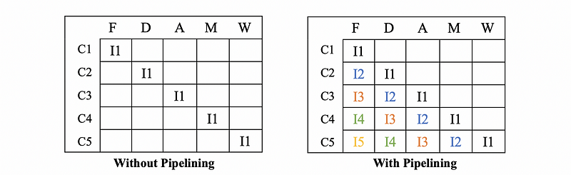
Suppose each phase takes equal time (20/5 = 4ns). Let’s calculate the latency and the throughput for these two different situations,
Without Pipelining,
- Latency: 20 ns
- Throughput: 1 / 20ns = 0.05 instructions per ns
With Pipelining,
- Latency: 20 ns
- Throughput: 1 / 4ns = 0.25 instructions per ns
This is quite similar to the oil pipeline.
(4) Pipeline Stalls and Flushes
We have mentioned that each of the 5 phases in a pipelining process takes 1 cycle to finish, so the CPI of the pipeline can be naturally calculated through 1 / 1 = 1 cycle per instruction. However, this value is not true in practice, and the CPIs are always larger than 1. There are 3 reasons for this,
- Initial Fill: we have talked that we have to full-fill the pipeline for the best performance initially because it will take longer for the first instruction compared with the others.
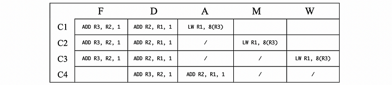
- Pipeline Stalls: even the pipeline is full-filled initially, the CPIs can still be larger than 1. In the design of pipelined computer processors, a pipeline stall is injected into the pipeline by the processor to resolve data hazards where the data required to process an instruction is not yet available. When a hazard occurs in a phase, the processor suspends the pipelining process for 1 cycle and redo this phase with a second cycle.
Let’s see an example of the following assembly code,
LW R1, 8(R3)
ADD R2, R1, 1
ADD R3, R2, 1
Because LW means to load from the memory, thus ADD R2, R1, 1 should wait until the LW command writes the data from the memory to the register (the W phase). There fore, ADD R2, R1, 1 has to wait for two cycles and this adds to the overall CPI.
In modern processors, pipeline stalls are all figured out in hardware. The hardware logic for figuring out forwarding and stalls looks at the instruction in the Decode stage. Note that a NOP is just an instruction with no side-effect, and this is different from the pipeline stalls.
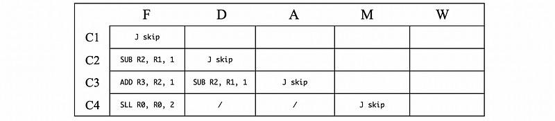
- Pipeline Flushes: The pipeline flush is another source that will cause the CPI higher than 1. Pipeline flushes are quite similar to the pipeline stalls, but it occurs when there’s a JUMP instruction. Let’s see the following assembly code,
J skip
SUB R2, R1, 1
ADD R3, R2, 1
skip:
    SLL R0, R0, 2
After we fetch a JUMP instruction, during the F/D/A phases, we don’t know the location that we are going to jump to. So the processor fetches the following two instructions SUB and ADD . After the ALU phase, we can then know where we are going to jump to, and this tells us that we should have fetched the instructions from somewhere else. So what happens now is called a pipeline flush. What we do is to convert these fetched instructions SUB and ADD into pipeline bubbles and then as the jump moves on, these two bubbles will also move on and cause a CPI larger than 1.
2. Pipeline Dependencies And Hazards
(1) Control Dependencies
Let’s say we have a program like this,
ADD R1, R1, R2
BEQ R1, R3, label
ADD R2, R3, R4
SUB R5, R6, R8
...
label:
    MUL R5, R6, R8'
    ...
The definition of control dependencies is that we can say the ADD and SUB … instructions after the BEQ have a control dependence of the branch instruction BEQ, because whether these instructions should be executed or not depend on the result of the BEQ instruction. Similarly, the MUL … instructions also have a dependence on the branch. So when we have a branch, all subsequent instructions that we execute have a control dependence on the branch. What this really means is that we don’t know whether we should be able to fetch these instructions until we figure out the branch.
let’s now see an example of the influence of the control dependencies. Suppose we have a 5-stage CPI with 20% branch/jump instructions, and it is estimated that slightly more than 50% of these branch/jump instructions are taken (meaning that they go somewhere else instead of just continuing). So what is the general overall CPI in this case?
Putting together all the information, we can know that about 10% (20% * 50%) of instructions in the program work as the branch/jump instructions. And based on our previous discussions of the pipeline flushes, each of these branch/jump instructions takes 2 idle cycles. Thus, the cycles per instruction can be then calculated by CPI = 1 + 10% * 2 = 1.2 .
In reality, most CPI is more than 5 stages (which means the CPI depth is larger than 5), this means the penalty of the idle cycles is larger than 2. However, we also have a technique that we are going to introduce called the branch prediction, which significantly reduces the branches or jumps that take the flushes. Thus, the percentage of this penalty will be reduced. Notice that the CPI depth can the branch prediction are related because when we have deeper CPIs, we have to use better branch predictions to reduce the penalty.
(2) Data Dependencies
The data dependency can also cause the pipeline stalls. Consider the following two instructions,
ADD R1, R2, R3
SUB R7, R1, R8
We can find out that the SUB instruction has a data dependence on the ADD instruction because its value of R1 is dependent on the result of the ADD instruction. This kind of relationship is called data dependence and it means that we can not just do the instructions as they have nothing to do with each other. There are many kinds of data dependencies,
- RAW (Read After Write) data dependency (or Flow data dependency): we read something after it has been written. So we have to wait for the written instruction and the order of these instructions need to be preserved. For example,
ADD R1, R2, R3
SUB R7, R1, R8
- WAW (Write After Write) data dependency (or Output data dependency): because we want to maintain the final value of a register, so we must keep the order of the instructions in case the value is rewritten by the other writing instructions. For example,
ADD R1, R2, R3
SUB R1, R7, R8
- WAR (Write After Read) data dependency (or Anti-data dependency): because we don’t want a write instruction to impact a read instruction right before it, so the order of these two instructions should be maintained. For example,
ADD R2, R1, R3
SUB R1, R7, R8
- True data dependency: Because the data in one register doesn’t exist until the previous instruction finished, so the order of these instructions must be preserved. The RAW dependency is actually a true dependency. For example,
LW R1, 0(R0)
SUB R7, R1, R8
- False data dependency: the WAW and WAR dependencies are also called the false dependency due to some reasons that we are going to introduce later.
(3) Dependencies and Hazards
We have known that the dependency is the property of the program alone and we can check whether two instructions have dependence between them without any regard to what the pipeline looks like. In a particular pipeline without bubbles in it, some dependencies will cause problems potentially and some dependencies cannot cause problems whatever. The situation when a dependence can cause a problem in the pipeline is called a hazard.
Our conclusion is that the false data dependency will not cause a hazard, while the true dependency can cause a hazard when there’s no bubble in a pipeline. Let’s see three examples of how it works. Suppose we have a 5-stage CPI,
#1. False WAW Dependency
ADD R1, R2, R3
MUL R1, R4, R5
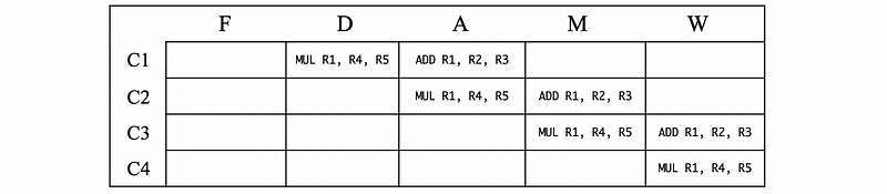
- In Cycle 1, the
MULis decoded and the sum of R2 and R3 is calculated - In Cycle 2, the product of R4 and R5 is calculated
- In Cycle 3, the value of sum is written to R1
- In Cycle 4, the value of product is written to R1
We can actually find out that, when there’s no bubble, the order of two writing instructions are maintained automatically. Thus, the WAW dependency won’t be a hazard.
#2. False WAR Dependency
MUL R1, R4, R5
SUB R4, R6, R7
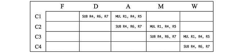
- In Cycle 1, the
SUBis decoded and the product of R4 and R5 is calculated - In Cycle 2, the subtraction of R6 and R7 is calculated
- In Cycle 3, the value of product is written to R1
- In Cycle 4, the value of subtraction is written to R4
Similarly, when there’s no bubble, the order of the reading and then writing instructions is maintained automatically. Thus, the WAR dependency won’t be a hazard.
#3. True RAW Dependency
SUB R4, R6, R7
DIV R10, R4, R8
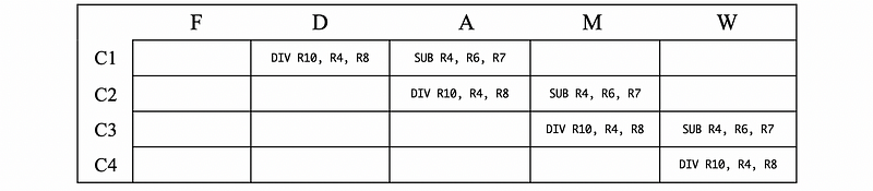
- In Cycle 1, the
DIVis decoded and the subtraction of R6 and R7 is calculated - In Cycle 2, the division of R4 and R8 is calculated
- In Cycle 3, the value of subtraction is written to R4
- In Cycle 4, the value of division is written to R10
Woah! We have a hazard here. In the cycle 2 and 3, the value in R4 is read at the first place, and then it is rewritten by the SUB instruction. However, what we want is that we want to use the result of R4 after the subtraction. This hazard occurs when a dependency results in the incorrect execution order of one or more instructions.
(4) Hazard Expectation for True Dependencies
You may consider that the true dependencies can cause hazards when there are no bubbles. However, when there are no bubbles, does the true dependencies necessarily cause the hazards? The answer is no and let’s see an expectation. Suppose we have the following program,
ADD R1, R2, R3
MUL R7, R4, R5
SUB R4, R6, R7
DIV R10, R5, R8
XOR R11, R1, R7
The XOR has 2 true data dependencies of R1 from the ADD instruction, and R7 from the MUL instruction. However, in this case, there will no hazards caused by R1 but there may be a hazard caused by R7. Why?
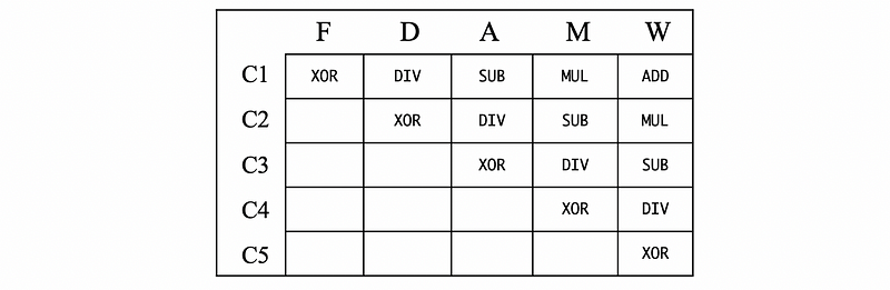
- In cycle 1, the
ADDinstruction writes to R1 before R1 is read byXOR, so the R1 cannot cause any hazards in this case. - In cycle 2, the
MULinstruction writes to R7 when theXORis reading from R7, so it is possible thatXORreads R7 after R7 is written byMUL, then there will be no hazards. However, it can also be possible thatXORreads R7 before R7 is written byMUL, then there will be a hazard. Thus, we can conclude that there may be a hazard caused by R7.
From the expectation instance above, we can conclude that, in a 5-stage pipeline, if there are 3 or more instructions between the writing (producing) instruction and the reading (consuming) instruction, then consuming instruction reads the register after the producing one has already written it. However, when there are no more than 2 instructions between the producing instruction and the consuming instruction, then it is possible that this RAW dependency is going to cause a hazard.
Note that we have to notice the process of reading the registers occurs during whether the DECODE stage or the ALU stage. In our conclusion above, we have assumed that this is during the DECODE stage. However, when the process of reading the registers happens during the ALU stage (or some other), the conclusion will be different.
(5) Handling the Hazards
Because we do not allow the pipelines to produce incorrect results, we need to handle only the situations that are hazards. Actually, we don’t really care about dependencies that can never become hazards. To handling a hazard, we have to do,
- Step 1. Detect the hazard situations
- Step 2. Find out whether it is caused by a control dependency or a data dependency
- Step 3–1. For control dependency, we use pipeline flushes to handle the hazard because the pipeline stall will not work for branching or jumping.
- Step 3–2. For data dependency, we can use stalls for handling the hazards instead of flushes (actually, we never use flushing for the data dependency). For some of the data dependencies, we can even fix the value read by the dependent instructions, and this is called forwarding. The forwarding means that instead of reading from the register, we directly use the result from the ALU in the last step because the value has already been calculated by the last instruction by ALU and it is just not written to the register. However, this method can be invalid if there are some instructions between them and the result of the ALU is replace by some other calculations. So if we want to use forwarding, we have to make sure our value exists somewhere in the pipeline, or we may have to choose the pipeline stalls and the cost is our CPI.
3. Pipeline Stages
We have used the 5-stage pipeline in most of the examples above. However, let’s talk about how many stages a pipeline should have. In the pipeline we have seen so far, the ideal CPI is 1. Actually, we are going to see that the ideal CPI should be smaller than 1 later in this series because they try to do more than 1 instruction per cycle.
What if we have more stages for our pipeline?
- More hazards: more instructions to be flushing, more stalls should be added, so the CPI increases because of the increasing penalty
- Less work per stage: if we have less work per cycle, then the cycle clock time (CCT) can be decreased. Thus, our clock can be speeded up.
Based on the Iron law, the have known that,

Let’s say that we have the same amount of instructions and our CPI goes up, but the cycle clock time drops. So the number of stages has to be chosen in a way that balances the CPI and the CCT.
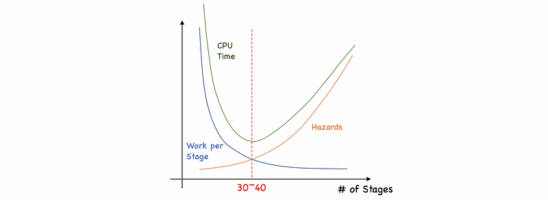
For modern processors, the optimized number of stages would be like 30 to 40 and this number of stages provides the best performance (speed). However, there are other concerns about the power. When we increase the frequency of our clock when decreases the clock time, the power consumption increases rapidly. So take both the performance and the power consumption into consideration, we will finally end up with a result of 10 to 15 stages in modern processors.
Sometimes you may find someone that is overclocking the processor, which means this guy wants to ignore the power concerns to achieve better performance with more stages.