High-Performance Computer Architecture 7 | Branch Prediction Part 1
High-Performance Computer Architecture 7 | Branch Prediction Part 1

1. Branch Penalty in a Pipeline
Let’s see the following code,
BEQ R1, R2, Label
A branch instruction like BEQ in the code above compares registers R1 and R2. And if they are equal, then we jump to the Label. This is usually implemented by having the difference between the next instruction’s PC and the PC that should be at the label in the immediate part of the instruction field. So effectively, if R1 and R2 are equal, the branch would just add the immediate operand to its current PC that is computed for the next instruction.
Thus, if R1 != R2 , then PC++ (only increment the PC, move 4 bytes). Else if R1 == R2 , then PC = PC + 4 + Imm (increment the PC and also add the immediate, move to the Label).
In the pipeline, we always assume (or predict) that the branch will not be working because we fetch the new instructions before we know the instruction is a branch (at the DECODE phase) and before we know whether or not it will branch (at the ALU phase).
Now there are two possibilities. If our prediction is right and the branch is not effective, then there will be no penalty. However, if we mispredict the result, the branch instruction (in our case, the BEQ instruction) will take 3 cycles because of the pipeline flushes (1 cycle for BEQ, 2 idle cycles for the penalty).
2. Disadvantage of Stalls after Branch Instead of Flushes
You can also see why it never pays to not fetch anything after the branch. If we don’t fetch anything after the branch until we are sure about what to fetch, then we are guaranteed to have two empty slots after the branch. So somehow in that case, regardless of whether we would have guessed correctly or not, we have a two-cycle penalty. Because we would rather have the 2-cycle penalty some of the time than all of the time, we would like to predict instead of stalling after all the branches.
Another thing that is important is that right after the FETCH stage, we don’t know the instruction is a branch instruction (we have just obtained the instruction word, which is a 4-byte value). So the instruction after the branch instruction must be fetched because we don’t even know whether it is a branch or not before the instruction is decoded.
3. Branch Prediction Requirements
Thus, if we want to improve the performance of our computer, we have to successfully predict whether our branches are taken or not and where they are going if the branches are taken.
What we have if we want to predict a branch instruction? At the FETCH stage where a prediction is needed, we only know the PC of the current instruction and what we want to predict is the PC of the next instruction to fetch. So our prediction must answer the following questions,
- Is this a taken branch? : If this is not a branch, then certainly it is not taken. If it is a branch, is it taken?
- What is the target PC? : If it is a taken branch, what is the target PC and where is this branch going?
We have to answer these two questions through our prediction.
4. Branch Prediction Accuracy
Our CPI can be written as 1 + penalty, which is the CPI we get with the ideal pipelining plus the overall penalty we pay because of the misprediction. The overall penalty can be calculated by the production of how often we have the mispredictions (this is determined by the predictor accuracy) and the penalty in terms of cycles we pay for each of these mispredictions (this is determined by the pipeline). Thus, the overall CPI can be written as,

Let’s see an example. Suppose 20% of all instructions are branches. For the first processor, the branch instructions are resolved in the 3rd stage, while for the second one, the branch instructions are resolved in the 10th stage. If we know the predictor accuracy for the branches is 50% and the accuracy for the other instructions is 100%. Then,
CPI for Processor #1: 1 + 20% * 50% * 2 = 1.2
CPI for Processor #2: 1 + 20% * 50% * 9 = 1.9
Similarly, if we change the predictor accuracy for the branches is 90% and the accuracy for the other instructions is 100%. Then,
CPI for Processor #1: 1 + 20% * 10% * 2 = 1.04
CPI for Processor #2: 1 + 20% * 10% * 9 = 1.18
Therefore, we can conclude that a better branch predictor will help us regardless of whether we have a shallow (or deep) pipeline. When we change the predictor from 50% to 90% branch accuracy, the speedup for the first processor is 1.2/1.04 = 1.15, while the speedup for the first processor is 1.9/1.18 = 1.61. As you can see, the deeper the pipeline, the more dependent it is on having a good predictor for good performance. In reality, we can actually have predictors significantly better than 90%, so we are still benefiting from this improvement.
5. Branch Prediction Benefit Example
Suppose we have a standard 5-stage pipeline with branches resolved in the 3rd stage. Let’s assume that this processor is a SAFE processor, which means that the processor fetches nothing until it is sure about what to fetch. If the processor now execute many iterations of the following program,
Loop:
    ADDI R1, R1, -1
    ADD  R2, R2, R2
    BNEZ R1, Loop
Suppose we have an IDEAL processor, which means that the predictor accuracy for the branch instruction is 100%, then what is the speedup between the ideal processor and the safe processor?
It is obvious that for the ideal processor, because all the branches are predicted successfully, then we actually pay no penalty for branches and the overall CPI for this processor is 1. To solve this problem, we also have to calculate the overall CPI for the safe processor, and this can be a little bit tricky.
Actually, for this safe processor, when in the fetch phase, we don’t know whether it is a branch instruction or not, so we will not fetch the next instruction until the end of the decode phase. Thus, the ADDI instruction and the ADD instruction will take 2 cycles (including 1 idle cycle to wait for the result of decoding). For the branch instruction BNEZ, it will take 3 cycles (including 2 idle cycles to wait for the result of decoding and to wait for the result of where to branch). So the overall CPI for this safe processor should be (2 + 2 + 3) / 3 = 2.33 and the speedup should be 2.33/1 = 2.33. We will discuss more of this in the next segment.
6. Refuse to Predict VS. Not-Taken Predictor
According to what we have seen in the example above, if we refuse to predict the branch instructions, a branch instruction will take 3 cycles and the other instructions will also take 2 cycles instead of only one cycle.
Let’s see a comparison, suppose we predict the branches with a not-taken predictor (means that by default, we assume that all the branches are not taken). Then a branch instruction will take 3 cycles (when the branch is actually taken) or 1 cycle (when the branch is finally not taken) and the other instructions will also take only 1 cycle.
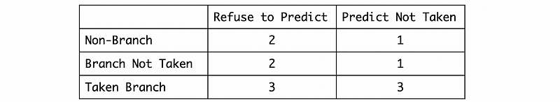
By this relationship, we can draw the conclusion that the predict not taken can always win over the refuse to predict. This is why every processor is going to do some sort of prediction even the prediction is simply to assume that the instructions are not taken by default.
7. The Simplest Predictor: Not-Taken Predictor
The not-taken predictor is actually the simplest predictor and now we would like to talk more about it. The predictor is the simplest because all it requires to do is to increase the PC. We know the PC from the instruction we fetch and we also know how big the instruction is (4 bytes), so we can simply increase the PC for this predictor.
The advantage of this predictor is that,
- It requires no memories
- It requires no other operations
Based on the rule of thumb, 20% of all the instructions are branches, so 80% of the time, this predictor must be correct because the instructions are simply not branches. For branches, a little more than 50% (we will use 60% as its value in this explanation) of branches are actually taken. Therefore, the proportion when this predictor is correct is 80% + 20% * (1 — 60%) = 88% and the incorrect proportion is 100% — 88% = 12% (or this can be calculated by 60% * 20% = 12%).
If we know the penalty of this pipeline, we can also calculate the impact on the overall CPI. The CPI will be 1 + 12% * penalty. Specifically, in a standard 5-stage pipeline, the penalty will be 2 and then the overall CPI should be 1.24.
8. Why we need other predictors?
We have seen that the not-taken predictor is simple and it predicts correctly with a prediction accuracy of 88%. So why do we need any better predictors? Let’s see the following table. Say we have two predictors, one is a standard not-taken predictor with an accuracy of 88%, and the other is an improved predictor with an accuracy of 99%,
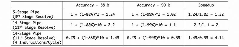
The larger the pipeline, the greater the penalty, especially when the branches are detected later in the pipeline and there are multiple instructions per cycle. This also means that there is a lot of waste from a misprediction, especially if it is a deep (more stages) and/or wide (more instructions per cycle) pipeline.
In the next section, we are going to talk about the predictors with better accuracy.