High-Performance Computer Architecture 8 | Branch Prediction Part 2
High-Performance Computer Architecture 8 | Branch Prediction Part 2

- The Better Predictor Using History
(1) Difficulties of Finding Better Predictors
We have seen that the not-taken predictor computes the next PC based on an increment of the current PC. Generally, when we have a predictor, it should compute the next PC based on a function f of the current PC. This can be written as,

If we can find some functions f that better predicts the next PC, then this predictor is going to have better performance. However, because all we know is the current PC, then probably you can not make a better prediction. To make a better prediction, we have to know,
- If the instructions is a branch?
- Is the branch taken?
- What is the offset field of the instruction? Because we want to get the offset to add to the current PC so as to form the next PC.
It is actually quite a pity that we actually don’t know anything about these after we fetch the instruction. So it seems like it is hopeless for us to get a better predictor. Is this true? Of course not!
(2) Better Prediction with History Information
Even though we don’t know anything about the current PC, however, we do know something about it based on its history. Assume that we have already known that the instruction is a branch and we want to know whether it is taken or not taken, we can use the history behaving to guess its next behavior. This method is based on the assumption that branches stand to behave the same way over and over again and this is actually what really happens. Still, we don’t know what the current branch is going to do, but we can what it did when it was executed a few previous times.
(3) The Definition of Branch Target Buffer (BTB)
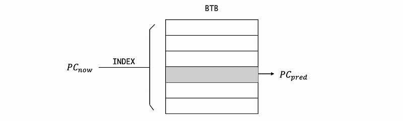
The simplest predictor that uses the history is called the branch target buffer (BTB) and what it does is that: it takes the current PC of the branch and uses that to index a table called BTB, and from the table, what will readout is our best guess for what the next PC will be. So during the fetch stage, the process seems like the following diagram.
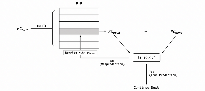
Another problem is how we can write to the table BTB. When we made a true prediction, the PC_pred would be exactly the same as PC_next, so we can just continue. However, if we made a wrong prediction (misprediction), then the current PC_pred value will be rewritten by the PC_next (the true value of this time). Note that the rewriting process requires the current PC PC_now as an index to the BTB. So next time we see this branch, we will get the correct prediction assuming it is going to jump to the same location.
(4) The Size of BTB
Because what we want is that in one cycle, we were given the current PC and then predict the PC based on the BTB, so it needs to have a single cycle latency. That means we want the size of BTB to be really small in order to finish the indexing in a single cycle.
However, each entry in the BTB needs to contain an entire instruction address. let’s say we are using 64-bit addressing and each entry takes up to 8 bytes. That means the size of the BTB can actually be really large!
So we cannot have a dedicated entry in the BTB for every possible PC address. In reality, it’s enough if we have enough entries for all the instructions that are likely to execute. For example, assume that we have a loop with 100 instructions, and after the first loop, the BTB will include all the instructions in the loop after which point we will keep finding what we need in the BTB.
(5) Mapping PCs to BTB Using LSB
Now that we have many PCs and we have to use each PC as an index of the BTB. So the question is how do we map each PC to an entry in the BTB? We have some requirements for this mapping function,
- Avoid Conflicts: or we will get the same entry given different PCs
- Simple Function: because any delay in computing the mapping function means that we need an even smaller BTB if we want to finish the whole thing in 1 cycle
The way we mapping the PC is, from the program counter (PC) which we are fetching, let’s say if the PCs are 64-bit values and we have 1024 entities in the BTB, then we can simply use the 10 least significant bits (LSB) as the index for our BTB. This mapping function is really fast because all we do is take the 10 bits without any calculation.
It is also important to know why the least significant 10 bits are used for indexing instead of the most significant 10 bits. Let’s think about an example of common PCs,
0x24A4: ADD
0x24A8: MUL
0x24AC: SLL
0x24B0: BEQ
If we mapping these instructions with the least significant 16 bits of the PC, we can find out that they can avoid conflicts because each of them is unique in the BTB and each of them can be direct to an entry. However, if we use the most significant 16 bits, the indexes will all be 24 and the entities can not be indexed through this value. So the nearby instructions, in this way, can not be mapping into a BTB.
(6) Mapping PCs to BTB: An Example
Let’s see an example now. Suppose our BTB has 1024 entries. If the instructions were 4-byte fixed, word-aligned and the program counters are 32-bit addresses. So which BTB entry is used for PC = 0x0000AB0C in hexadecimal value?
Note that when we say the instructions were 4-byte fixed, word-aligned, we are meaning that all the instructions should take 4 bytes (4-byte fixed) and all the addresses would be divided by four (word-aligned). When the addresses must be divided by 4, the least significant two bits of a PC must be 00. Here is a reference table shows us the relations between the least significant bits and all the alignments,
Alignments             Least significant bits
Byte-alignment                       anything
Halfword-alignment                          0
Word-alignment                             00
Doubleword-alignment                      000
Now let’s review our question. 0x0000AB0C ends with a binary value of 101100001100 and we have known that the least significant 2 digits are always 00 . So in this case, we should ignore these two values and grab the 10 bits before these two bits in order to map into 1024 entries of the BTB. Thus, the index we will have in this case is 1011000011 and this should be converted to the hexadecimal value 0x2C3 .
2. 1BP and 2BP for the BHT Predictor
(1) Direction Prediction Through BHT
The BTB is going to tell us when a branch is taken, where should it go based on the historical results. However, we also have to predict whether or not a branch is taken. This is called the direction prediction and we are going to have a table that we will call a branch history table or a BHT to deal with it.
We will take the current PC of the instruction, grab the LSB and then index it into the table BHT. So what you can see here is quite similar to index into a BTB. However, the entry in a BHT is much smaller. The simplest BHT predictor will simply have 1 bit per entry that tells us whether this is a not-taken branch (with bit = 0) or this is a taken branch (with bit = 1).
If 0 is gotten from this bit, then we can simply increase the PC (PC++) because this branch will not be taken. However, if 1 is gotten from this bit, then we use the BTB to tell us where to go. Just like we were updating the BTB, we can update this value once we dissolve this branch. If the resolution shows that it is a taken branch, we will put 1 in the BHT, and then we rewrite the destination address into the BTB if needed. If the resolution shows that it is a not-taken branch, we will put 0 in the BHT, and the BTB will not be updated.
Because the simplest BHT only requires 1 bit per entry, so the size of the BHT can be quite large. Thus, we can have lots of instructions avoiding conflicts between instructions that commonly execute while still reserving the small BTB which has much fewer entries only for branches in that code.
(2) Problems With 1-Bit BHT Predictors (1BP)
We have said in the last section that the simplest BHT predictor has 1 bit per entry that tells us whether an instruction is a taken branch or not. It seems that this 1-bit BHT works well in some of the situations for,
- always taken branches: without penalty except for the first time. After the first time misprediction, there will be no more mistakes and the BHT will start to predict “taken”.
- always not-taken branches: because the BHT starts from a state of not-taken, then there’s not going to be a misprediction for the first time prediction. So there will be generally no penalty in this situation.
However, the problems occur when there’s the following situation,
- taken > not taken or not taken > taken: this predictor doesn’t work well when there is an insignificant proportion pattern of taken (or not taken) against the other one. The penalties appear when the instructions change their taken state. Because one instruction state surpasses the other one with an insignificant scale, the penalty can not be simply ignored.
Let’s see an example of this. Suppose we have the following sequential taken state of one branch instruction,
Taken State    T T T T N T T T T
Prediction     ✓ ✓ ✓ ✓ ✗ ✗ ✓ ✓ ✓
From this example, we can find out that each anomaly results in two mispredictions, one for the anomalous behavior and once more for the normal behavior that follows the anomaly.
There are more problems with this 1-bit preditor in a short loop because typically in a short loop, we are going to have two mispredictions while exiting the loop (mispredict the last iteration) and entering the loop (mispredict the very first iteration).
There is even a more server situation and this predictor works pretty bad when the proportion of taken is close to the proportion of not taken (taken ≈ not taken) for a branch instruction. We are going to leave it here and focus more on it later.
(3) The Definition of 2-Bit BHT Predictors (2BP)
The predictor that fixes the problems of the 1-bit BHT predictor is called a 2-bit predictor. It can also be written as 2BP or 2BC, which stands for the 2-bit counter.
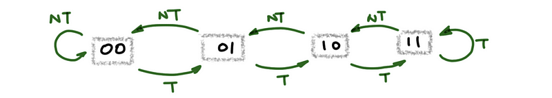
Literally, there are 2 bits in the 2BP. The more significant bit is called the prediction bit and a value of 1 means that we will predict take, while a value of 0 means that we will predict not taken. The less significant bit is called the hysteresis (or conviction) bit and it tells us how sure are we when we are making the prediction by the more significant bit. A value of 0 means we strongly believe that the prediction is right, while a value of 1 means that we are not so sure with the prediction. Thus,
00      Strong Not Taken
01      Weak Not Taken
10      Weak Taken
11      Strong Taken
Recall, we can draw the outcome of 1BP as follows,

While 2BP is more like a double confirmation when we change the state. The next prediction will not be changed until there’s a double confirmation that tells us it is quite convincing to believe that the taken state is really changed instead of some anomalous outcomes. The workflow is actually like,
(4) Initial State of 2-Bit BHT Predictors (2BP)
For 1BP, we always start from the not-taken state because there are only 2 states, and also there are more non-taken-branch instructions. So it would be a good idea if we start from the not-taken state (bit = 0).
However, things are more complex when we use 2BP because now we have 4 states. Suppose, similarly, we would like to start from the not-taken state and now we have two choices. We can either start from the strong not-taken state or the weak not-taken state. Which one is better?
Let’s think about starting from the strong not-taken state first,
Start in Strong State:
- if always not taken
00 00 00 00
NT NT NT NT
✓  ✓  ✓  ✓
- if always taken
00 01 10 11
T  T  T  T
✗  ✗  ✓  ✓
Based on the result above, we can know that if we start from the strong not-taken state, we pay nothing when the branch is always not-taken. However, we will have 2 mispredictions when the branch is always taken.
Let’s think about starting from the strong not-taken state first,
Start in Weak State:
- if always not taken
01 00 00 00
NT NT NT NT
✓  ✓  ✓  ✓
- if always taken
01 10 11 11
T  T  T  T
✗  ✓  ✓  ✓
Based on the result above, we can know that if we start from the weak not-taken state, we pay nothing when the branch is always not-taken. However, we will have only 1 misprediction when the branch is always taken.
Now, it may seem like that we should initialize the 2BP with the weak not-taken state. But there’s actually an expectation that can provide disaster results if we do so. Let’s think about an alternative state,
Start in Strong State:
00 01 00 01
NT T  NT T
✓  ✗  ✓  ✗
Start in Weak State:
01 10 01 10
NT T  NT T
✗  ✗  ✗  ✗
Woah! We can find out that all the predictions are wrong if we start from the weak state and it can really be a disaster for us. However, fortunately, the situation of an alternative state is rare and an always state is much more common. So to initialize the 2BP with the weak not-taken state is still a good idea.
But you can also notice that in reality, it will not influence too much whether we choose to start from a strong state or a weak state. This is because the strong state initialization pays for the always taken state while the weak state initialization pays for the alternate state. So in general, the overall accuracy of the branches is affected very little by the initialization state.
(5) Problems When More Bits of BHT Predictors
We have seen that we improved the predictor a lot by adding 1 bit to each entry of the BHT predictors. Why don’t we have more bits? Well, it is possible for us to improve the accuracy of the predictors by adding more bits when the anomalous outcomes come in streaks. However, because each branch will have a corresponding entry in BHT, the more bits we have in the BHT, the higher the cost of memory would be. Based on the fact that the situation of anomalous outcomes come in streaks is not very often, 2BP is enough for most of the cases.
3. History-Bit Count Predictor
(1) Predictors for the Alternate States
Let’s recall the following problem. When we have alternate states, either 1BP or 2BP works really bad. For example,
#1: N T N T N T N ...
#2: N N T N N T N ...
However, this is predictable for any human being and we can easily capture the pattern of these alternate states. The only problem is that the 1BP and 2BP can not learn from this pattern and guess the next state correctly. In fact, we can predict the next branch through historical patterns. For example, if we set the rules,
For #1:
- N -> T
- T -> N
For #2:
- NN -> T
- NT -> N
- TN -> N
then we can predict the alternate patterns correctly.
(2) 1-Bit History With 2-Bit Count Predictor
Let’s see how we can build a predictor that learns from the historical patterns. Instead of 1 bit or 2 bit for each entry in the BHT, each of these entries is assigned with 5 bits including a history sign, a 2BC for the not-taken branch, and a 2BC for the taken branch,
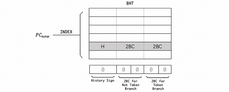
When the last branch is taken, then the history sign is assigned by 1, or it will be assigned to 0 if the last branch is not taken. If the last branch is taken (history sign = 1), then we read the 2BC from the “2BC for taken branch”. If the last branch is not taken (history sign = 0), then we read the 2BC from the “2BC for not taken branch”.
Let’s see a stable state for predicting the alternate state pattern N T N T N ...,

When the last branch is not taken, then the history sign would be assigned to 0 and we will use strong taken as our 2BC predictor state. So the next one must be taken. Similarly, when the last branch is taken, then the history sign would be assigned to 1 and we will use strong not taken as our 2BC predictor state. So the next one must be not taken. By this means, we can finally get a predictor that can work for the alternate states.
However, this can not be working for the alternate state pattern N N T N N T N ... and there will be a misprediction for 1/3 of all these branch instructions. We are not going to calculate the result here and I am quite sure that you can also achieve this result. So what we can do if we want to build a predictor for this pattern? It is easy to guess that we actually need a 2-bit history with 2-bit count predictor.
(3) 2-Bit History With 2-Bit Count Predictor
When we have 2 bits for the history sign, we actually have 4 historical states. For each of these historical states, we have to assign a 2BC for tracing the taken information. Thus,

For alternate states N N T N N T N ..., the final stable state is,

We are not going to prove this because it is quite obvious. Note that we can’t generate a historical state of TT , so it doesn’t matter what is the value of the last two bits. Because the last 2-bit BC never gets used but we must have it, we actually wasted some of the memories.
(4) N-Bit History With 2-Bit Count Predictor
Now, let’s see some general conclusions. Suppose we have N history bits, then
- It will correctly predict all pattern of
length ≤ N + 1. Note that the number of patterns is the number of iterations in a loop. For example, a branch loop ofNNNNNNNNThas 9 patterns andN = 8is enough for predicting these patterns. - There should be
2^N2BC predictors - The memory cost per entry should be
N + 2 * (2^N)per entry, so when N increases, the cost increases exponentially - Most of the 2BCs will be wasted if we have a large N
So the general solution for this kind of problems is that,
Step 1. Spot the main loop and count the iterations n for this loop. A loop with n iterations can also be written as (NN...NT)* with n-1 N (means branch not taken).
Step 2. Calculate the # of the patterns by N = n — 1.
Step 3. Calculate the number of 2BCs by 2^N.
Step 4. Calculate the memory cost per entry by N + 2 * (2^N) .