High-Performance Computer Architecture 9 | Branch Prediction Part 3
High-Performance Computer Architecture 9 | Branch Prediction Part 3

- History-Based Predictor With Shared Counters
(1) Continue with the Wasted 2BCs
In the previous section, we have encountered the case that with N + 1 patterns and now let’s talk about how to reduce the waste by having fewer than 2 to the nth counter and yet have a long history.
The motivation for this is that with N-bit history,
- we will need
2^N2BCs per entry - only about
N2BCs are actually used, and the other 2BCs are wasted
So the idea here is to share these 2BCs between entries instead of dedicating 2^N 2BC counters to each entry.
(2) Conflict Concerns of the Shared Counters
We will have a pool of 2BCs that entries will then use, but it is also possible that different entries with different program counters with different histories will end up using the same 2BC. So there’s a possibility of conflict, but if we have enough of these 2BCs because each entity doesn’t need too many of them, we will usually have very few conflicts.
(3) Shared Counters Implementation
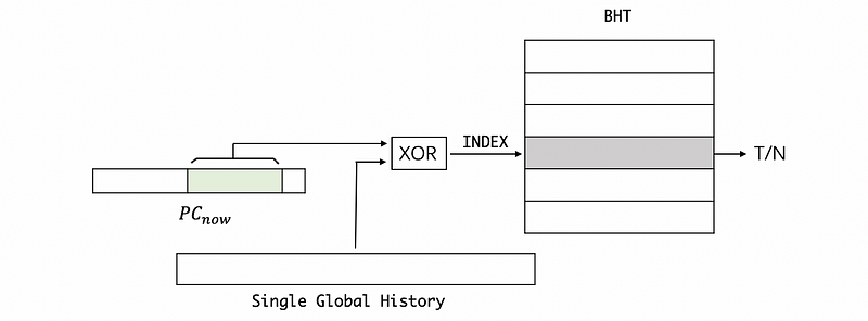
So how can we implement the shared counters? The answer is as follows. We have the program counter PC and we take some of the lower bits. Then we use these bits to index into a table called pattern history table (PHT) which is a table that keeps the history bits alone with the current branch. This can also be treated as only the history sign part in the previous BHT. To grab some 2BCs for this history, we take the history from this table and then XOR it with the bits from the PC. The result from this XOR operation can be then used to index the branch history table (BHT). Note that this BHT is not the same as the previous one and each entity in this BHT is only a single 2BC. Then, this entry will tell us whether or not we should be predicting taken or not taken.

Note that it is possible for another PC to XOR with its history and to index us the same 2BC in the BHT. But we can ignore this overlap because it is quite rare to happen.
Now let’s do some calculations to see how much we have reduced the memory cost. Suppose we grab 11 bits from the current PC for indexing and our history has 10 patterns. Based on what we have discussed, a history of 9 bits is enough for representing this pattern.
For the previous BHT without shared counters,
- Memory cost = memory cost per entry * # of the entries, so,
Memory cost = [N + 2 * (2^N)] * (2^n) = [9 + 2 * (2^9)] * (2^11)
= 2115584 bits = 25.86 KB
For the PHT and BHT with shared counters,
- Memory cost = (memory cost per entry in PHT + memory cost per entry in BHT )* # of the entries, so,
Memory cost = (N + 2)* (2^n) = (9 + 2) * (2^11)22528 bits = 2.75 KB
=
Based on this calculation, we can find out that the memory cost reduces about 9/10 if we use the shared counters. So this is a huge progress for us and we can tolerate some conflicts in order to achieve this improvement.
2. PShare and GShare
(1) The Definitions of Private Share and Global Share
When we have shared counters, we actually separate the history bits (in PHT) and the 2BCs (in BHT).
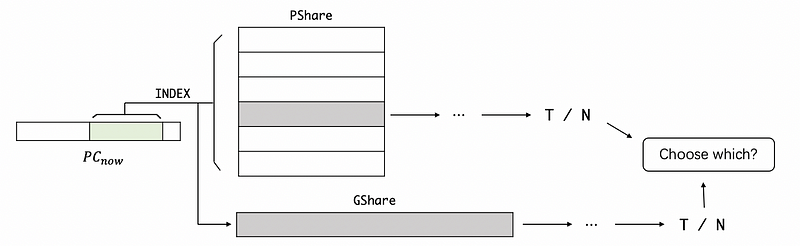
A private share (PShare) predictor has a private history for each branch and each branch should have its own history in the PHT. The PShare predictor also has shared counters so that different histories and different branches might map to the same counter. The PShare predictor is good for things whenever the branch on previous behavior is predictive of its future behavior (i.e. Even-odd behavior like (NT)* or loops with few iterations).
A global share (GShare) predictor has a single global history for all branches (or you can think about a PHT with only one entry). The GShare predictor also has shared counters so that different histories and different branches might map to the same counter. So what we have is now we actually have a single global history that we can use for all branches.
The GShare is good from the correlated branches like the two if statements in the following code. If we have the history of the first line, we will be sure to make the right prediction when executing the second line.
if (shape == square) { ... }
if (shape != square) { ... }
(2) PShare Vs. GShare: An Example
Now let’s do some calculations to see the difference between a PShare predictor and a GShare predictor. Suppose we have the following C program,
for (int i = 100; i != 0; i--)
    if (i % 2)
         n += i;
This can be compiled to
Loop:
    BEQ R1, 0, Exit
    AND R2, R1, 1
    BEQ R2, 0, Even
    ADD R3, R3, R1
Even:
    ADD R1, R1, -1
    B Loop
Exit:
Suppose we want good accuracies on all branches, then how many bits of history should the PShare and GShare have respectively?
Note that we have three branches in this program.
For PShare,
- The first
BEQhas a pattern ofNN...NTand only the last branch is taken. So it doesn’t matter whether we have a history or not for this branch. - The second
BEQhas an odd-even pattern ofNTNT...and we need to have at least 1 bit of history to predict this branch - The last loop
Bis an unconditional loop ofTT..., so this means that the branch will always be taken. Thus, it doesn’t matter whether we have a history or not for this branch.
Therefore, the minimum size of PHT should be 1 bit per entry.
For GShare, we have to consider the three branches together for the overall history. The first branch BEQ should be N until the last bit, the second NEQ should be N or T based on the history, and the last branch B must be taken T. Thus, the branches follow,
N N T N T T N N T N T T ...
Based on this record, we can know that the minimum size of history we need to make an accurate prediction is 3 bits. The reason is,
NNT -> N
NTN -> T
TNT -> T
NTT -> N
TTN -> N
TNN -> T
This example gives us an insight that the GShare predictor has a longer history than the PShare.
(3) PShare or GShare: Which One to Choose?
We have known that GShare can do some correlated branches, while PShare takes a shorter history than GShare. So which one should we choose for our processor? Many earlier processors choose between either PShare or GShare, but very quickly, people figured out that we can actually choose both of them.
This brings us to an idea called tournament predictor.
3. Tournament Predictor and Hierarchical Predictor
(1) The Definition of Tournament Predictor
Let’s say we have two predictors, and we have known that PShare is better for some branches, while GShare is better for some other branches. So the best idea is to use the PShare for some branches, and GShare for the others. To implement that, we will use our current PC for indexing into both of the predictors. Then we will generate two results and we have to choose which one to use.
The idea for a tournament predictor is to use a meta-predictor which is just an array of 2BCs. We also use the current PC to index there, but the entry of a tournament predictor is actually going to tell you which of the two predictors is going to give a more accurate prediction for that branch. So we use the 2-bit result from the tournament predictor for choosing which predictor should we selected.
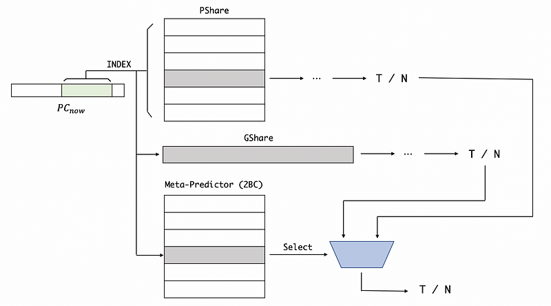
Note that the PShare and GShare predictors are trained just like before, while the meta-predictor should be trained in a different way. If two predictors are both correct or both wrong, then the meta-predictor doesn’t change anything. If the first predictor is correct, then this predictor counts down. If the second predictor is correct, then this predictor counts up.
00 Strongly Choose the 1st Predictor
01 Weakly Choose the 1st Predictor
10 Weakly Choose the 2nd Predictor
11 Strongly Choose the 2nd Predictor
(2) The Definition of Hierarchical Predictor
The tournament predictor typically combines two good predictors, while a hierarchical predictor combines a good predictor and an ok predictor (which is not so good). This is because if we do 2 good predictions for every branch just use one of them and each of the good predictors costs you a lot.
The tournament predictor updates both of the predictors on each decision, while the hierarchical predictor update only the ok predictor on each decision and the good predictor will be updated only if the ok predictor is not good.
In practice, the hierarchical predictor always wins.
(3) Hierarchical Predictor: An Example
We will now have a look at the Pentium M predictors as our example. This processor includes,
- 2BC Predictor (Cheap)
- Local History Predictor
- Global History Predictor
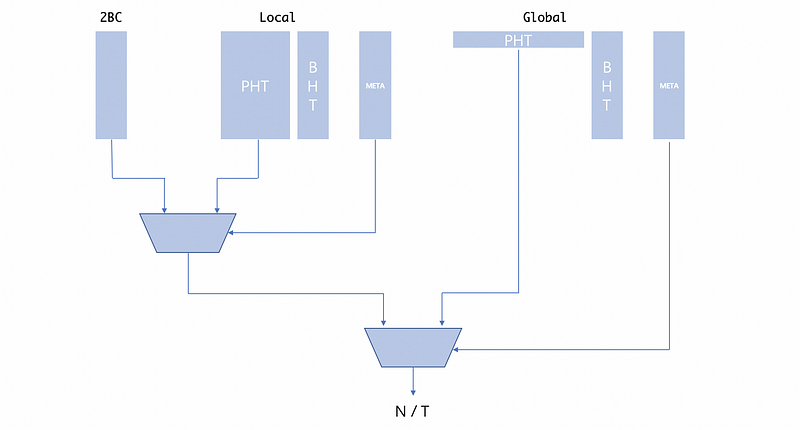
Note that the meta-predictor in the hierarchical predictor stores the matching tags which decide whether or not to use a better predictor. In the beginning, all the meta-predictor would be empty and there will be no matching tags. If 2BC mispredict the result, then some bits of this branch address will be added to the matching tags of the local predictor, so next time, it will use the local predictor for prediction. When to use the local predictor and the global predictor has the same rules.
4. Return Address Stack (RAS) Predictor
(1) Problems for Predicting Function Returns
We have seen that there are several types of branches that we need to predict.
For conditional branches,
- we need to predict the direction (taken or not taken). We have already seen many branches that can make good predictions of this.
- if the branch is taken, we also need to predict the target address. A simple BTB predictor will be fine because we always have the same target.
For unconditional jumps and function calls,
- the direction is always taken so this is trivial
- the target will either jump to a label or call a specific function, so BTB will be just fine
For function returns,
- the direction is always taken so this is trivial
- the target of a function returns will often difficult to predict. Usually, we create a function and then call this function from multiple locations in the program. In this case, BTB will be our bad choice and we have to use RAS for this case.
(2) The Definition of Return Address Stack (RAS) Predictor
The return address stack (RAS) is a separate predictor dedicated to predicting the function returns. The way it works is that the RAS is actually a small stack close to the branch instructions (for finishing the predictions in 1 cycle). As we execute the program when we have a function call, we will push the return address. When we have the return instruction, we will pop the address and then move the pointer. Actually, it can be seen as address storage instead of a prediction.
There is a problem with RAS because the RAS is a really small stack and it can be exceeded by calling new functions easily. If our RAS is full, we have two strategies,
- don’t push anything in order to preserve our address on RAS
- wrap around by continue writing to the RAS. The wrap-around approach is better because the function returns follow the rule of LIFO (last in first out). So it is more useful for us to keep the latest function call.
(3) How to Know a Return?
A remaining problem is that how could we know whether a branch is a function return branch or not in the fetching stage? Because the instruction is not decoded yet but we have to decide whether or not to pop from the RAS. We have two methods for knowing this,
- Using a 1BP predictor
This will be a very accurate predictor because it is significantly possible for a PC to be a function return branch if it was a function return branch before
- Using predecoding
We will see that the processor really contains a cache that stores the instructions fetched from the memory. This works by when on fetching from the memory, we decode enough of the instruction to know whether that is a return or not. This predecoding is quite tricky because it seems like we did a decoding phase when we got the branch instructions from the memory and put them into the cache.