High-Performance Computer Architecture 19 | Compiler for Improving ILP, Tree Height Reduction…

Series: High-Performance Computer Architecture

High-Performance Computer Architecture 19 | Compiler for Improving ILP, Tree Height Reduction, Instruction Scheduling, Loop Unrolling, and Function Inlining

Review

We have completed the discussion that if we want to improve the IPC, we have to implement the out-of-order execution for the load/store instructions and non-load/store instructions. And in order to deal with the exceptions, we developed the ROB. However, to implement more than one instruction per cycle, we will discuss how the compiler can help.

2. Compiler For ILP

(1) The Definition of Instruction-level Parallelism (ILP)

Instruction-level Parallelism (ILP) is a family of processor and compiler design techniques that speed up execution by causing individual machine operations, such as memory loads and stores, integer additions, and floating-point multiplications, to execute in parallel.

(2) Limited ILP Problem

In a real program, if we have a long chain of dependent instructions, we can do very little ILPs because we can really execute only one instruction at a time. However, with the help of a compiler, we will see that the compiler might help us actually avoid these kinds of dependence chains.

(3) Limited “Window” Problem

There is another problem because of this long dependence chain. The hardware will have a limited window into the program. For example, there might be independent instructions, so an ideal processor might be able to achieve good ILP under the program. But because these independent instructions are far apart, a real processor simply can not see those instructions because it runs out of the ROB space before it reaches those instructions that are independent. As we will see, the compiler can help us put these independence instructions closer to each other, so that the IPC achieved by the processor is closer to the available ILP.

3. Compiler ILP Techniques

(1) Tree Height Reduction

One of the examples of a technique to actually improve the ILP of the program is tree height reduction. Let’s say we need a program that has to add the values in R1, R2, R3, and R4, and then store the final result in R5,

R5 = R1 + R2 + R3 + R4

One way to get that result is,

ADD R5, R1, R2
ADD R5, R5, R3
ADD R5, R5, R4

However, this form of dependence chain is quite long. We can find out that the second instruction depends on the first one, and the third instruction depends on the second one. So all of these instructions have to be done one after another.

The tree height reduction is that the compiler figures out that instead of adding one number at a time to get the sum and thus creating a chain of dependencies, what we can do is to group the computation in the following way for the same result,

R5 = (R1 + R2) + (R3 + R4)

So in this way, the assembly should be,

ADD R5, R1, R2
ADD R8, R3, R4
ADD R5, R5, R8

We can know that the third instruction depends on both the first instruction and the second instruction. However, the first instruction is independent of the second instruction, so they can be executed parallelly. So without the tree height reduction, we need three cycles to execute this program, while with the tree height reduction, we only need two cycles because the first instruction and the second instruction can be executed in parallel.

(2) Instruction Scheduling

We will look now at the instruction scheduling in the compiler. Here’s what can happen. Let’s first look at the following program,

Loop:
    LW  R2, 0(R1)
    ADD R2, R2, R0
    SW  R2, 0(R1)
    ADD R1, R1, 4
    BNE R1, R3, Loop

Assume that we have a very simple processor that can only look at the very next instruction and can only execute 1 instruction in a cycle. So it does not really have the reservation stations and the out-of-order execution. Suppose that the add instruction takes 3 cycles for execution, the load instruction takes 2 cycles, and the store takes only 1 cycle. So the schedule of the program above will be,

LW  R2, 0(R1)
STALL
ADD R2, R2, R0
STALL
STALL
SW  R2, 0(R1)
ADD R1, R1, 4
STALL
STALL
BNE R1, R3, Loop

This is because even though the instruction ADD R1, R1, 4 can be executed right after the instruction LW R2, 0(R1) , the processor can only look at the very next instruction and it didn’t know that we have ADD R1, R1, 4 . Thus, in general, we have to wait for 10 cycles to complete this program.

The instruction scheduling means that the compiler will move the independent instructions to build a new schedule. In this new program, the compiler will move the instruction ADD R1, R1, 4 after the LW R2, 0(R1) , and because the value in R1 will be changed by an increment of 4, thus, we have to reduce the 4 for the instruction SW R2, 0(R1).

Loop:
    LW  R2, 0(R1)
    ADD R1, R1, 4
    ADD R2, R2, R0
    SW  R2, -4(R1)
    BNE R1, R3, Loop

So the schedule for the new program above will be,

LW  R2, 0(R1)
ADD R1, R1, 4
ADD R2, R2, R0
STALL
STALL
SW  R2, -4(R1)
BNE R1, R3, Loop

We can find out that only 7 cycles are required now. Note that if we have a better processor, the first instruction and the second instruction can even be executed in the same cycle parallelly.

(3) Instruction Scheduling: Another Example

Let’s see another example of instruction scheduling. Suppose we have the following program,

LW  R1, 0(R2)
ADD R1, R1, R3
SW  R1, 0(R2)
LW  R1, 0(R4)
ADD R1, R1, R5
SW  R1, 0(R4)

Suppose that we have a processor with the following features,

1 instruction / cycle, in-order execution
load instruction takes 2 cycles
add instruction takes 1 cycle
store instruction takes 1 cycle

Then the as-is instruction schedule should be as follows,

LW  R1, 0(R2)
STALL
ADD R1, R1, R3
SW  R1, 0(R2)
LW  R1, 0(R4)
STALL
ADD R1, R1, R5
SW  R1, 0(R4)

After the instruction scheduling, we can move the second load instruction LW R1, 0(R4) to the front of this program. However, because this instruction will write to the R1 and then cause a data conflicting problem, we have to rename the register of this instruction. So after the instruction scheduling, the program will be,

LW  R1, 0(R2)
LW  R10, 0(R4)
ADD R1, R1, R3
ADD R10, R10, R5
SW  R1, 0(R2)
SW  R10, 0(R4)

Note that the add instruction and the store instruction will also be moved to make the program even more structured.

(4) Instruction Scheduling and If-Conversion

Let’s first recall what is the if-conversion. The if-conversation is a technique for us to avoid the branch instructions. This means that we will calculate both ways of taken the branch and not taken the branch, and then use a conditional move to decide which one to use finally.

Then we have to think about how the instruction scheduling is going to interact with the if-conversation. Actually, we can conclude that the if-conversation is going to help with the scheduling. Why? Let’s think about a branch model. In the following model, we can hardly conduct the instruction scheduling because if we mispredict the branch, all the things we have done for the scheduling are then useless because we never go to that branch.

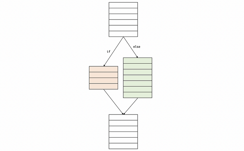
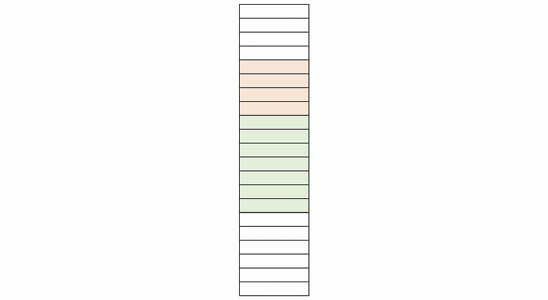
However, after if-conversion, both of the branches are executed and we can then conduct the instruction scheduling because this is a branch-free code and we don’t have to worry about the branch not taken.

(5) If-Convert Looping

Could the if-conversation work for the loop so that we can then conduct instruction scheduling? To answer this question, let’s see an example here. Similarly, suppose we still have the looping program above,

Loop:
    LW  R2, 0(R1)
    ADD R2, R2, R0
    SW  R2, 0(R1)
    ADD R1, R1, 4
    BNE R1, R3, Loop

Assume that our processor is an in-cycle, 1 IPC processor with 2 cycles for a load instruction, 2 cycles for an add instruction, and 1 cycle for a store instruction. By what we have discussed before, before the instruction scheduling, we can have the following schedule for each loop,

LW  R2, 0(R1)
STALL
ADD R2, R2, R0
STALL
SW  R2, 0(R1)
ADD R1, R1, 4
STALL
BNE R1, R3, Loop

However, after the instruction scheduling, we will then have the program,

Loop:
    LW  R2, 0(R1)
    ADD R1, R1, 4
    ADD R2, R2, R0
    SW  R2, -4(R1)
    BNE R1, R3, Loop

And the schedule for each loop should be,

LW  R2, 0(R1)
ADD R1, R1, 4
ADD R2, R2, R0
STALL
SW  R2, -4(R1)
BNE R1, R3, Loop

While in each of the loops, we can find that there is still one stall. If we think about using the if-conversion, we can actually fill in this stall with some instructions after the loop (because the branch will be eliminated). But this method has a problem. The loop is not really suitable for if-conversion because every time we have a new iteration, we will have a new predicate. After several loops, we will have many predicates that can not be dealt with easily. For example, if we are executing a million iteration loop, only in one loop we will break out, so almost a million iterations will have a useless predicate. Thus, the program will be very slow.

Now, we want to find some instructions to fill in the stalls but we don’t really want to do the if-conversion of a loop. Is there anything else we can do? Well, the answer is the loop unrolling.

(6) Loop Unrolling

Loop unrolling creates a loop with fewer iterations by having each iteration do the work of two or more iterations. To understand the loop unrolling, let’s first see an example of C. Suppose we have the following program,

for(i=1000;i!=0;i--) 
   a[i] = a[i] + s;

Then the compiled assembly code is,

Loop:
  LW   R2, 0(R1)
  ADD  R2, R2, R3
  SW   R2, 0(R1)
  ADDI R1, R1, -4
  BNE  R1, R5, Loop

Where R1 stores the address for the a[i] and R3 stores the value of s .

Unrolling once means that we will do two iterations at a time in the loop (it is a common mistake to think that unrolling twice is to do two iterations at a time in the loop), this is to say that the C program will then be,

for(i=1000;i!=0;i-=2) 
   a[i] = a[i] + s;
   a[i-1] = a[i-1] + s;

Then the compiled assembly code should be,

Loop:
  LW   R2, 0(R1)
  ADD  R2, R2, R3
  SW   R2, 0(R1)
  LW   R2, -4(R1)
  ADD  R2, R2, R3
  SW   R2, -4(R1)
  ADDI R1, R1, -8
  BNE  R1, R5, Loop

(7) Loop Unrolling for ILP

Now let’s discuss how does the unrolling loop improve the ILP. The ILP is improved in two ways,

decrease the overall number of instructions

In the last example, before the loop unrolling, we have to run 5 instructions 1,000 times, which means that we'll have 5,000 instructions in general. However, after unrolling once, we only have to run 8 instructions 500 times, and this means that we are going to have 4,000 instructions generally. We have this improvement by reducing what is called the looping overhead. In the case of unrolling once, we do twice of the work but we only do have to apply half of the looping overheads.

Recall that the execution time of a program is the number of the instructions times the CPI times the cycle time per instruction. And because we have reduced the number of the instructions with almost no impact on the cycle time per instruction, so the overall execution time is going to be determined by the CPI and the number of instructions.

Now, let’s see what happens to the CPI.

decrease the overall CPI

Assume that we have a 4-issue, in-order processor (meaning that it is only able to look at the next 1 instructions to see what can be executed) with perfect branch prediction.

=> Case 1: No unrolling, without scheduling

Suppose we have the following instructions (as we have talked about in the loop unrolling),

Loop:
  LW   R2, 0(R1)
  ADD  R2, R2, R3
  SW   R2, 0(R1)
  ADDI R1, R1, -4
  BNE  R1, R5, Loop

We can calculate the CPI of this program by the following table,

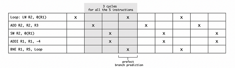
Because we can execute all these 5 instructions in 3 cycles, the overall CPI for this program is 3/5 = 0.6.

=> Case 2: No unrolling, with scheduling

In the previous case, we didn’t take instruction scheduling into consideration. After instruction scheduling, we will have,

Loop:
  LW   R2, 0(R1)
  ADDI R1, R1, -4
  ADD  R2, R2, R3
  SW   R2, 4(R1)
  BNE  R1, R5, Loop

Then the looping diagram would be,

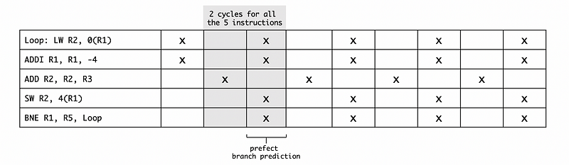
Because we can execute all these 5 instructions in only 2 cycles, the overall CPI for this program is 2/5 = 0.4.

=> Case 3: Unrolling once, without scheduling

As we have discussed, if we conduct unrolling once, we will then have the program,

Loop:
  LW   R2, 0(R1)
  ADD  R2, R2, R3
  SW   R2, 0(R1)
  LW   R2, -4(R1)
  ADD  R2, R2, R3
  SW   R2, -4(R1)
  ADDI R1, R1, -8
  BNE  R1, R5, Loop

So the resulting diagram will be,

Because we can execute all these 8 instructions in 5 cycles, the overall CPI for this program is 5/8 = 0.625.

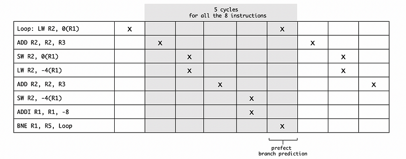
=> Case 4: Unrolling once, with scheduling

Let’s see what will happen if we conduct a scheduled unrolling once. The program would be,

Loop:
  LW   R2, 0(R1)
  LW   R10, -4(R1)
  ADD  R2, R2, R3
  ADD  R10, R10, R3
  ADDI R1, R1, -8
  SW   R2, 8(R1)
  SW   R10, 4(R1)
  BNE  R1, R5, Loop

The resulting diagram would be,

Because we can execute all these 8 instructions in 3 cycles, the overall CPI for this program is 3/8 = 0.375.

So in conclusion, we can find out that the loop unrolling can not only reduce the number of the instruction and the overall CPI. So that the execution time of the processor can be reduced.

(8) Loop Unrolling Downsides

So far, unrolling seems like a pretty good thing and we tend to do unrolling all the time. However, there are some downsides to enrolling, and let’s discuss them now.

Code Bloat: code bloat is the production of program code that is perceived as unnecessarily long. You can see that with fewer unrollings, we can have a shorter code, while the code size grows rapidly with the number of the underlings with much more unrollings we do
Can’t handle the situation that the unknown number of interaction: for example, this could be a while loop and we may not sure about how many iterations we would have. So it is impossible for us to implement unrollings
Can’t handle the situation that the number of iteration is not n times the number of unrollings: if this happens, that means we have to break the loop in its middle and this is difficult to implement

We may talk about these sections above in a compiler series.

(9) Function Inlining

The inlining is another technique for the functions. The inlining for functions is similar to unrolling for loopings. Inlining involves removing the function call and just replacing it with the body of the function. Let’s see an example here, suppose we have the following program,

some work ...
prepare function parameters
call function
other work ...

And we assume that the function call is supposed to be,

function: ADD Rn, A0, A1
RET

Then if we conduct the function inlining, the overall code can be,

some work ...
ADD R7, R7, R8
other work ...

You can find out that we don’t have to do the preparation for the parameters anymore.

The benefits of the inlining are that,

eliminate call/return overheads (fewer instructions)
instruction scheduling can be conducted for the whole code (lower CPI)

Thus, in general, the overall execution time will be reduced by a lot and the performance will be improved.

The downsides of inlining are as follows,

Again, code bloat: we know that the same function may be called for several times in a program, and if we conduct the inlining, the code size grows rapidly. So the application results in a lot more code than the original calling and returning code.

3. Other IPC Enhancing Compiler Techniques

There are some other techniques that can be used for compilers to improve the IPC. The present series do not require these techniques, but we may learn more about them in the compiler series. These techniques are,

software pipelining: covert some instructions to avoid dependencies
trace scheduling: the common path will be extracted for scheduling. Note that because we use the common path for most cases, we may have to execute some fixing code if we have a less common path