High-Performance Computer Architecture 21 | Midterm Review
High-Performance Computer Architecture 21 | Midterm Review

- Metrics and Evaluations
(1) Dynamic Power (Active Power)

where,
Cis the total capacitanceV²is the voltage square and this is the power supply voltagefis the clock frequencyαis the activity factor
(2) Overall Power

(3) Fabrication Yield

(4) Latency and Throughput

(5) Speedup

(6) Mean Speedup (Geometric Mean)

(7) Iron Law of Performance

(8) General Iron Law of Performance

Note that different kinds of instructions can have different cycles.
(9) Amdahl’s Law

(10) Lhadma’s Law
While trying to make the common case fast, don't make the uncommon case worse.
Example 1-1. (Amdahl’s Law) Booth’s algorithm is used to perform signed binary multiplication. The machine that uses Booth’s algorithm to perform a multiplication executes 129 cycles and the machine with the hardware multiplier takes 15 cycles per multiple. Given that 5% of all the instructions in a given benchmark are 32-bit binary multiplications. Calculate how much faster after the hardware machine is enhanced by Booth’s algorithm.
Ans:
Speedup_mul = 129/15 = 8.6
Speedup_frac = 1/(0.95+0.05/8.6) = 1.0462
Example 1-2. (Iron Law and Amdahl’s Law) Your company currently uses the “High RISC” processor by RISCy Solutions. It is a 2GHz processor with an average CPI of 1.5. RISCy Solutions has just come out with two new processors which you are to compare and select the best performer.
Triple the RISCis a three pipelined machine that also runs at 2GHz, and maintains the same CPI as the High RISC. It is estimated that one-third of your code can use all three pipelines and another third can use two pipelines. For an n-pipelined processor, the ideal speedup is n.RISCily Fastis a 5GHz single processor, that due to its speed encounters a larger memory penalty. When the cache misses (5% of the time) on memory accesses (40% of all instructions), it incurs a penalty of 50 cycles more than the original High RISC processor. In all other ways, it is identical to the High RISC.
Ans:
// speedup for "Triple the RISC"
Speedup_1 = 1/(1/3 + (1/3)/3 + (1/3)/2) = 18/11 = 1.6364
// speedup for "RISCily Fast"
Speedup_2 = Latency(High RISC) / Latency(RISCily Fast)
          = CPUtime_HR / CPUtime_RF
          = IC * CPI_HR * CCT_HR / (IC * CPI_RF * CCT_RF)
          = 1.5 * (1/2) / (CPI_RF * (1/5))
          = 1.5 * (1/2) / ((CPI_HR + 50*5%*40%) * (1/5))
          = 1.5 * 5 / (2.5 * 2)
          = 1.5
Because Speedup_1 > Speedup_2, we should choose Triple the RISCExample 1-3. (Amdahl’s Law and Diminishing Returns)
Memory operations currently take 20% of execution time.
- a first new widget speeds up 80% of the memory operations by a factor of 4
- a second new widget then speeds up 30% of the memory operations by a factor of 2 after the first widget
What is the total speed up after these two widgets?
Ans:
// Note that we have to take diminishing returns into consideration
// first widget
Speedup_1 = 1/((1-20%) + (1-80%)*20% + 80%*20%/4) = 1/0.88 = 1.1364
// calculate the diminishing return
Original:  |-------80%--------|--20%--|
Frac_non_mem = 0.8/0.88 = 91%
Frac_mem = 1-Frac_non_mem = 9%
After:     |-------91%--------|9%|
// second widget
Speedup_2 = 1/(91% + 9%*70% + 9%*30%/2) = 1/0.9865 = 1.0137
// total speedup
Speedup = Speedup_1*Speedup_2 = 1.1520 = 1.15
Example 1-4. (Amdahl’s Law)
Use Amdahl’s law to prove the conclusion that it is important to keep a system balanced in terms of the performance of the I/O (memory operation) speed and the CPU (non-memory operation) speed.
Ans:
Assume that we have 10% of the I/O operation time and 90% of the CPU operation time. Suppose the CPU operation has speedups of 10, 100, and 1,000. Then the total speedup of the system will be,
Speedup_1 = 1/(10% + 90%/10) = 5.2632
Speedup_2 = 1/(10% + 90%/100) = 9.1743
Speedup_3 = 1/(10% + 90%/1000) = 9.9108
We can find out that the system performance will be restricted by the I/O operations if we don’t balance the performance.
Example 1-5. (Iron’s Law)
Suppose we have a 1-ns clock cycle unpipelined processor that uses 4 cycles for the ALU operations, 5 cycles for the branches, and 4 cycles for the memory operations. Assume that we have a program that has 50% ALU operations, 35% branches, and 15% memory operations.
Now we can develop this processor by the clock skew and pipeline setups, the developed processor with one pipeline adds 0.15 ns of overhead to the clock. Ignore the latency impact, how much speed up in the instruction execution rate will we gain from a pipeline?
Ans:
// Unpipelined Processor
average_CPI_un = 4*50% + 5*35% + 4*15% = 4.35
// Developed Processor
CPI_pip = 1
// Speedup
Speedup = IC*average_CPI_un*CCT_1/(IC*CPI_pip*CCT_2)
        = 4.35*1 / (1*(1+0.15))
        = 4.35 / 1.15
        = 3.7826
2. Pipeline
(1) 5-Stage Model
- Fetch
- Decode
- ALU
- Memory Access
- Write Registers
(2) Dependency
When an instruction is dependent on the outcome from another instruction, these instructions have a dependency.
(3) Control Dependencies
When an instruction is dependent on the outcome of a branch decision, these instructions are said to have a control dependence.
(4) Data Deependendices
When an instruction needs data from another instruction that is called a data dependence.
(5) True Dependency, Flow Dependency, RAW Dependency
The read-after-write (RAW) dependency.
(6) False Dependency, Name Dependency
The write-after-write (WAW) dependency and the write-after-read (WAR) dependency.
(7) Hazard
A hazard is created when there is a dependency between instructions and they are close enough that the overlap caused by pipelining would change the order of access to the dependent operand.
- Control hazards are created when an instruction fetch depends on some branches under execution.
- Data hazards are true dependencies that result in incorrect execution of the program.
(8) Stall
A pipeline stall is a delay (NOP) in the execution of an instruction in order to resolve a hazard.
(9) Flush
A pipeline flush means that when the mispredict occurs (the incorrect branch is taken), then all the incorrect instructions that we have fetched must be flushed from the pipeline by replacing them with NOPs.
(10) Ideal CPI
Suppose we have an N-issue (means that we can execute N instruction in a cycle) ideal processor (means no penalty for misprediction), the ideal CPI is,

Note that if we have a pipeline with 5 stages, it doesn’t mean that we have 5 pipelines.
(11) Real CPI
Because the processor is not perfect, so the real CPI ≠ ideal CPI. We have to take penalties into our consideration,

(12) Misprediction Penalty
Sometimes we want to calculate the penalty (wasted cycles) per misprediction. Theoretically, this can be calculated by,

However, in practice, this should be calculated by

(13) Forwarding
The forwarding means that instead of reading from the register (after the writing stage), we directly use the result from the ALU stage (for the non-memory instructions) or the Memory access stage (for the memory operations). However, it can only supply the data in the next cycle.
(14) Branch Delay Slot
The branch delay slot is caused because the branch would not be resolved until the instruction has worked its way through the pipeline.
Example 2-1. (Dependencies and Hazards) Specify TRUE or FALSE to all the following statements.
- Dependencies are caused by both the program and the pipeline.
- Hazards are caused by both the program and the pipeline.
- Not all true dependencies will result in a hazard.
- Not all hazards are caused by true dependencies.
Ans:
F       // Only by the program
T
T
T       // can also be caused by control dependencies
Example 2–2. (Data Dependencies) Specify TRUE or FALSE to all the following statements.
- Only flow dependencies require data being transmitted between instructions
- The name dependencies can not cause the hazards
- The name dependencies can be dealt with by register renaming
- The flow dependencies can be dealt with by out-of-order execution
Ans:
T
T
T
T
Example 2–3. (Handling Hazards, Forwarding) Suppose we have the following code fragment,
Loop:
    LD   R1, 0(R2)
    ADDI R1, R1, #1
    SD   R1, 0(R2)
    ADDI R2, R2, #4
    SUB  R4, R3, R2
    BNEZ R4, Loop
Answer the following questions, and note that we assume that one iteration ends for the execution stage of the branch instruction.
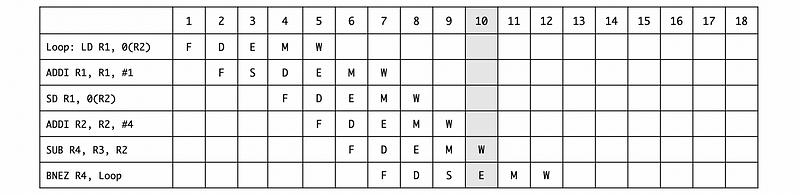
a. Draw the timing of this instruction sequence for a 5-stage pipeline for one iteration without forwarding. Assuming that registers can be r/w in the same cycle.
Ans:
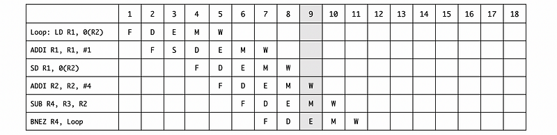
b. Draw the timing of this instruction sequence for a 5-stage pipeline for one iteration with forwarding. Assuming that registers can be r/w in the same cycle.
Ans:
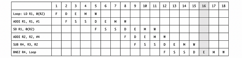
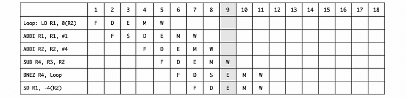
c. Suppose we have a timing of this instruction sequence for a 5-stage pipeline for one iteration as follows,
Note that the BNEZ instruction has one delay slot. Rewrite the code to fill in the slot and then draw the timing with forwarding.
Ans:
The point is that any instruction in the branch delay slot will get executed regardless of whether the branch is taken, even though it appears that the instruction will only be executed when the branch is not taken. So the code can be rescheduled to,
Loop:
    LD   R1, 0(R2)
    ADDI R1, R1, #1
    ADDI R2, R2, #4
    SUB  R4, R3, R2
    BNEZ R4, Loop
    SD   R1, -4(R2)
So what we want to do is take one of the existing instructions that would have been executed before the branch, and instead execute it during the delay caused by the branch. The reason why SD was chosen is that no other instruction in the loop depends on that instruction, until the next iteration.
3. Branch Prediction and Precidcation
(1) Rule of Thumb
Branches account for 20% of all instructions.
(2) Prediction Accuracy

(3) Refuse-to-Predict Predictor: no prediction
- For non-branch operations: 2 cycles
- For branches: 3 cycles
(4) Not-taken Predictor: always predict not taken
- For non-branch operations: 1 cycle
- For not-taken branches: 1 cycles
- For taken branches: 3 cycles
(5) Branch Target Buffer (BTB): predict by history branch PC
A table mapping the current branch PC number to the target PC. It is only accessed when the BHT says the instruction is a taken branch.
- Least Significant Bits (LSB) indexing
Note that the not-taken predictor takes no branches.
(6) Branch History Table (BHT)
The branch history table (BHT) is used to determine if the branch is taken or not taken.
(7) 1 Bit Predictor (1BP)
The BHT stores a 1-bit history for each branch.
1 == Taken
0 == Not Taken
(8) 2 Bit Predictor (2BP)
The BHT stores a 2-bit history for each branch.
00 == Strongly Not Taken
01 == Weakly Not Taken
10 == Weakly Taken
11 == Strongly Taken
(9) History-Based Predictor
We have to use a history-based predictor because the patterns can be learned.
(10) 1-Bit History 2-Bit Predictor/Counter (1BH2BP/BC)
// History Bit
0 == Choose the 1st 2-bit counter
1 == Choose the 2nd 2-bit counter
// 1st 2-bit counter
00 == Strongly Not Taken
01 == Weakly Not Taken
10 == Weakly Taken
11 == Strongly Taken
// 2nd 2-bit counter
00 == Strongly Not Taken
01 == Weakly Not Taken
10 == Weakly Taken
11 == Strongly Taken
(11) 2-Bit History 2-Bit Predictor/Counter (2BH2BP/BC)
// History Bit
00 == Choose the 1st 2-bit counter
01 == Choose the 2nd 2-bit counter
10 == Choose the 3rd 2-bit counter
11 == Choose the 4th 2-bit counter
// 1st 2-bit counter
00 == Strongly Not Taken
01 == Weakly Not Taken
10 == Weakly Taken
11 == Strongly Taken
// 2nd 2-bit counter
00 == Strongly Not Taken
01 == Weakly Not Taken
10 == Weakly Taken
11 == Strongly Taken
// 3rd 2-bit counter
00 == Strongly Not Taken
01 == Weakly Not Taken
10 == Weakly Taken
11 == Strongly Taken
// 4th 2-bit counter
00 == Strongly Not Taken
01 == Weakly Not Taken
10 == Weakly Taken
11 == Strongly Taken
(11) N-Bit History 2-Bit Predictor/Counter (NBH2BP/BC) Requirements
- Can predict patterns of length
N+1 - Cost
N+2*2^Nbits per entry
(12) Shared Counters
Because the cost of the history-based predictors is high and most of the counters are wasted, we use the shared counters in a BHT to reduce the cost of the predictor.
(13) Pattern History Table (PHT)
Because all the histories are going to use the same BHT for shared counters to reduce the cost, we can then split the BHT and store the pattern history in a table call the pattern history table (PHT).
(14) PShare (Local History Predictor)
PHT with entries for different pattern histories. This is good for small loops and predictable short patterns.
(15) GShare (Global History Predictor)
PHT with an entry for one global pattern history. This is good for correlated branches.
(16) Tournament Predictor
A tournament predictor combines two good predictors (i.e. PShare and GShare). It uses a meta predictor to choose between these two good predictors.
(17) MetaPredictor
A predictor for choosing between two good predictors.
00 == Strongly GShare
01 == Weakly GShare
10 == Weakly PShare
11 == Strongly PShare
(18) Hierarchical Predictor
A hierarchical predictor combines a good predictor and an okay predictor (i.e. PShare and 2BP predictor). The good predictor is only updated when the okay predictor is incorrect, so it saves the cost.
(19) Return Address Stack (RAS) Predictor
The RAS is a small stack (i.e. with only 4 entries) used to store the return address of the functions.
(20) Predication
Predication is doing the work of both directions and then choosing the correct one and throwing away the incorrect path work.
(21) If-Conversion
The if-conversion technique means that we are going to use conditions instructions for these two directions, such as MOVC and MOVZ.
(22) Full Predication
The full predication means that instead of using a conditioning move, we can conditional bits to every instruction for telling us what is the condition.
Example 3-1. (Predictors and Mispredictions) Consider the following MIPS code,
ADDR   LW R2, #0                // v = 0
       LW R3, #16
       LW R4, #0                // i = 0
       LoopI:
0x11C    BEQ R4, R3, EndloopI
         LW  R5, #0             // j = 0
       LoopJ:
0x124    BEQ  R5, R3, EndloopJ
         ADD  R6, R5, R4        // j+i
         ANDI R6, R6, #3        // (j+i)%4
0x130    BNE  R6, R0, EndIf     // skip if (j+i)%4 != 0
         ADD  R2, R2, R5        // v += j
       EndIf:
         ADDI R5, R5, #1
0x13C    BEQ  R0, R0, LoopJ
       EndloopJ:
         ADDI R4, R4, #1
0x144    BEQ  R0, R0, LoopI
       EndloopI:
a. Rewrite the code in C.
b. If we use an always-taken predictor, determine the exact number of branch mispredictions.
c. Note that the MIPS instructions always start at word-aligned addresses, so the two least significant bits are never used to index the BHT. If we use a one-bit predictor with an 8-entry BHT, and assume that all predictor entries start out with zero values, determine the exact number of branch mispredictions.
d. Note that the MIPS instructions always start at word-aligned addresses, so the two least significant bits are never used to index the BHT. If we use a local history predictor with 8 entries. Each entry has a 2-bit local history and four 2-bit counters. All history bits and 2-bit counters start out with zero values. Determine the exact number of branch mispredictions.
a. Ans:
v = 0;
for (i = 0; i < 16; i++) {
   for (j = 0; j< 16; j++) {
      if ((i+j)%4 != 0) continue;
      v += j;
   }
}
b. Ans:
Because this branch is predicted as always-taken, then the misprediction happens when,
- i = 0~15
- j = 0~15
- (i + j) % 4 = 0
Note that we don’t have to consider the last two branches because they are always taken.
For the first case, because the instruction BEQ R4, R3, EndloopI is executed 17 times and the last time it is taken. So the number of misprediction is 16.
For the second case, because the instruction is executed both in the loop for i and the loop for j , so it is executed 16*17 times. And because in each of the last iteration of the loop for j, it will be taken, the number of misprediction is 16*16 = 256 times.
For the last case, we have to consider the case when (i + j) % 4 == 0 . Both variable i and variable j can be chosen from 0 to 15, so,
i        j
----     --------------------
0        0     4     8     12
1        3     7     11    15
...      ...
15       1     5     9     13
Thus, the misprediction for this case is 16*4 = 64.
In conclusion, the exact number of branch mispredictions is 16 + 256 + 64 = 366.
c. Ans:
The 1-bit predictor 8-entry BHT at the beginning should be,
INDEX            PREDICTOR
-----------      -------------
000              0
001              0
010              0
011              0
100              0
101              0
110              0
111              0
The five branches are,
0x11C    BEQ R4, R3, EndloopI
0x124    BEQ R5, R3, EndloopJ
0x130    BNE  R6, R0, EndIf
0x13C    BEQ  R0, R0, LoopJ
0x144    BEQ  R0, R0, LoopI
Because we have a word-aligned LSB indexing (which means the last two bits should be ignored), the mapping rules should be
Address       Binary               LSB (3bits)
---------     ---------------      ----------------
0x11C         0001 0001 1100       111
0x124         0001 0010 0100       001
0x130         0001 0011 0000       100
0x13C         0001 0011 1100       111
0x144         0001 0100 0100       001
As a result, both 0x11C and 0x13C will be mapping to the 111 entry in the BHT, both 0x124 and 0x144 will be mapping to the 001 entry in BHT, and finally, 0x130 will be mapping to the 100 entry in the BHT.
Now, let’s first consider the 111 entry. This entry will be used for both 0x11C and 0x13C . For the branch 0x11C , it will be,
N N N N N N N N N N N N N N N N T
Or we could write it as,
{N}*16 TAlthough the branch 0x13C seems to branch all the time, there will be some mispredictions because it uses the same BHT entry with 0x13C . So, for each of the iteration for i, it will be,
T T T T T T T T T T T T T T T T
Or we could write it as,
{T}*16So in general, the overall branches would be,
{N {T}*16}*16 TThis is also to say that we have,
|---------------- 17*16 ------------------|
N T....T N T....T ... ... N T....T N T....T T
  |-16-|   |-16-|           |-16-|   |-16-|
By this diagram, we can find out that we have 31 mispredictions for this entry, 1 for the first Taken, and 15 times of conversion of Taken-Not Taken-Taken. So in summary, there would be 1+15*2 = 31 mispredictions for this case.
Similarly, for 001 entry in the BHT, 0x124 will be executed 16*17 times and in the branching status will be,
{N N N N N N N N N N N N N N N N T}*16Or we could write it as,
{{N}*16 T}*16For the 0x144 branch, we can know it is always taken but because it is written to the same entry of 0x124 , it will also cause some mispredictions,
T T T T T T T T T T T T T T T T
Because it will be executed after every 17 iterations of j, then the overall branching status for the 001 entry should be,
{{N}*16 T T}*16This is also to say that we have,
|------------------ 16 * 18 -----------------|
N .... N T T N .... N T T ... ... N .... N T T
|--16--|     |--16--|             |--16--|
By this diagram, we can find out that we also have 31 mispredictions for this entry, 1 for the first Taken, and 15 times of conversion of Taken-Not Taken-Taken. So in summary, there would be 1+15*2 = 31 mispredictions for this case.
In the end, let’s consider the entry 100 only for the branch 0x130 . This is simpler because we only have to consider only one branch. For this branch, as we have discussed before, it has a pattern of,
{N T...T N T...T N T...T N T...T}*16Or we could write it as,
{N T...T}*64Or, we can make it easier for us to find the mispredictions by,
N T...T {N T...T}*63So in summary, the mispredictions for this case is 1+63*2 = 127.
And in conclusion, the overall number of mispredictions should then be 31 + 31 + 127 = 189.
d. Ans:
The 2BH-2BC BHT at the beginning should be,
INDEX      Hist      2BC-0     2BC-1     2BC-2     2BC-3
-----      -----     -----     -----     -----     -----
000        00        00        00        00        00
001        00        00        00        00        00
010        00        00        00        00        00
011        00        00        00        00        00
100        00        00        00        00        00
101        00        00        00        00        00
110        00        00        00        00        00
111        00        00        00        00        00
As we have discussed, 0x11C and 0x13C will share the 111 entry, 0x124 and 0x144 will share the 001 entry, and 0x130 will use the 100 entry.
For the 111 entry, the pattern would be,
{N {T}*16}*16 TFor the 001 entry, the pattern would be,
{{N}*16 T T}*16For the 100 entry, the pattern would be (note that the sequence of NTTT is not solid),
{N T T T}*64Let’s discuss them one by one. Firstly, let’s talk about the 111 entry,
- the first
N {T}*16iteration,
For the first status (N), there will be nothing and we will predict it correctly,
INDEX      Hist      2BC-0     2BC-1     2BC-2     2BC-3
-----      -----     -----     -----     -----     -----
000        00        00        00        00        00
001        00        00        00        00        00
010        00        00        00        00        00
011        00        00        00        00        00
100        00        00        00        00        00
101        00        00        00        00        00
110        00        00        00        00        00
111        00        00        00        00        00
For the second status (T), we will mispredict it,
INDEX      Hist      2BC-0     2BC-1     2BC-2     2BC-3
-----      -----     -----     -----     -----     -----
000        00        00        00        00        00
001        00        00        00        00        00
010        00        00        00        00        00
011        00        00        00        00        00
100        00        00        00        00        00
101        00        00        00        00        00
110        00        00        00        00        00
111        00        01        00        00        00
For the third status (T), we will mispredict it,
INDEX      Hist      2BC-0     2BC-1     2BC-2     2BC-3
-----      -----     -----     -----     -----     -----
000        00        00        00        00        00
001        00        00        00        00        00
010        00        00        00        00        00
011        00        00        00        00        00
100        00        00        00        00        00
101        00        00        00        00        00
110        00        00        00        00        00
111        01        01        01        00        00
For the fourth status (T), we will mispredict it,
INDEX      Hist      2BC-0     2BC-1     2BC-2     2BC-3
-----      -----     -----     -----     -----     -----
000        00        00        00        00        00
001        00        00        00        00        00
010        00        00        00        00        00
011        00        00        00        00        00
100        00        00        00        00        00
101        00        00        00        00        00
110        00        00        00        00        00
111        11        01        01        00        01
For the fifth status (T), we will mispredict it, because the 2BC needs to be confirmed twice,
INDEX      Hist      2BC-0     2BC-1     2BC-2     2BC-3
-----      -----     -----     -----     -----     -----
000        00        00        00        00        00
001        00        00        00        00        00
010        00        00        00        00        00
011        00        00        00        00        00
100        00        00        00        00        00
101        00        00        00        00        00
110        00        00        00        00        00
111        11        01        01        00        10
For the 6th status (T), we will predict it correctly,
INDEX      Hist      2BC-0     2BC-1     2BC-2     2BC-3
-----      -----     -----     -----     -----     -----
000        00        00        00        00        00
001        00        00        00        00        00
010        00        00        00        00        00
011        00        00        00        00        00
100        00        00        00        00        00
101        00        00        00        00        00
110        00        00        00        00        00
111        11        01        01        00        11
For the 7th~17th status (T), we will predict them correctly.
- the second
N {T}*16iteration,
For the 18th status (N), we will mispredict it,
INDEX      Hist      2BC-0     2BC-1     2BC-2     2BC-3
-----      -----     -----     -----     -----     -----
000        00        00        00        00        00
001        00        00        00        00        00
010        00        00        00        00        00
011        00        00        00        00        00
100        00        00        00        00        00
101        00        00        00        00        00
110        00        00        00        00        00
111        11        01        01        00        10
For the 19th status (T), we will mispredict it,
INDEX      Hist      2BC-0     2BC-1     2BC-2     2BC-3
-----      -----     -----     -----     -----     -----
000        00        00        00        00        00
001        00        00        00        00        00
010        00        00        00        00        00
011        00        00        00        00        00
100        00        00        00        00        00
101        00        00        00        00        00
110        00        00        00        00        00
111        10        01        01        01        10
For the 20th status (T), we will mispredict it, because the 2BC needs to be confirmed twice,
INDEX      Hist      2BC-0     2BC-1     2BC-2     2BC-3
-----      -----     -----     -----     -----     -----
000        00        00        00        00        00
001        00        00        00        00        00
010        00        00        00        00        00
011        00        00        00        00        00
100        00        00        00        00        00
101        00        00        00        00        00
110        00        00        00        00        00
111        01        01        10        01        10
For the 21st status (T), we will predict it correctly,
INDEX      Hist      2BC-0     2BC-1     2BC-2     2BC-3
-----      -----     -----     -----     -----     -----
000        00        00        00        00        00
001        00        00        00        00        00
010        00        00        00        00        00
011        00        00        00        00        00
100        00        00        00        00        00
101        00        00        00        00        00
110        00        00        00        00        00
111        11        01        10        01        11
For the 22nd~34th status (T), we will predict them correctly.
- the third
N {T}*16iteration,
For the 35th status (N), we will mispredict it,
INDEX      Hist      2BC-0     2BC-1     2BC-2     2BC-3
-----      -----     -----     -----     -----     -----
000        00        00        00        00        00
001        00        00        00        00        00
010        00        00        00        00        00
011        00        00        00        00        00
100        00        00        00        00        00
101        00        00        00        00        00
110        00        00        00        00        00
111        11        01        10        01        10
For the 36th status (T), we will mispredict it, because the 2BC needs to be confirmed twice,
INDEX      Hist      2BC-0     2BC-1     2BC-2     2BC-3
-----      -----     -----     -----     -----     -----
000        00        00        00        00        00
001        00        00        00        00        00
010        00        00        00        00        00
011        00        00        00        00        00
100        00        00        00        00        00
101        00        00        00        00        00
110        00        00        00        00        00
111        10        01        10        10        10
For the 36th status (T), we will predict it correctly,
INDEX      Hist      2BC-0     2BC-1     2BC-2     2BC-3
-----      -----     -----     -----     -----     -----
000        00        00        00        00        00
001        00        00        00        00        00
010        00        00        00        00        00
011        00        00        00        00        00
100        00        00        00        00        00
101        00        00        00        00        00
110        00        00        00        00        00
111        01        01        11        10        10
- For the other iterations, we will only mispredict the Not-taken branch (the first branch in each iteration).
So in summary, the number of mispredictions, in this case, should be 22, because,
|   1-st iter   | | 2-nd iter | | 3rditer | |  other 13 iters |
N T T T T T ... T N T T T ... T N T T ... T N T ... T N T ... T
o x x x x o ... o x x x o ... o x x o ... o x o ... o x o ... o
So the number of mispredictions for the entry 111 should be 4+3+2+1*13 = 22.
Secondly, let’s talk about the 001 entry, it has the pattern of,
{{N}*16 T T}*16- the first
{N}*16 T Titeration,
For the 1st status (N), we will predict it correctly,
INDEX      Hist      2BC-0     2BC-1     2BC-2     2BC-3
-----      -----     -----     -----     -----     -----
000        00        00        00        00        00
001        00        00        00        00        00
010        00        00        00        00        00
011        00        00        00        00        00
100        00        00        00        00        00
101        00        00        00        00        00
110        00        00        00        00        00
111        00        00        00        00        00
For the 2nd status (N), we will predict it correctly,
INDEX      Hist      2BC-0     2BC-1     2BC-2     2BC-3
-----      -----     -----     -----     -----     -----
000        00        00        00        00        00
001        00        00        00        00        00
010        00        00        00        00        00
011        00        00        00        00        00
100        00        00        00        00        00
101        00        00        00        00        00
110        00        00        00        00        00
111        00        00        00        00        00
For the 3rd status (N), we will predict it correctly,
INDEX      Hist      2BC-0     2BC-1     2BC-2     2BC-3
-----      -----     -----     -----     -----     -----
000        00        00        00        00        00
001        00        00        00        00        00
010        00        00        00        00        00
011        00        00        00        00        00
100        00        00        00        00        00
101        00        00        00        00        00
110        00        00        00        00        00
111        00        00        00        00        00
For the 4th~16th status (N), we will predict them correctly.
For the 17th status (T), we will mispredict it,
INDEX      Hist      2BC-0     2BC-1     2BC-2     2BC-3
-----      -----     -----     -----     -----     -----
000        00        00        00        00        00
001        00        00        00        00        00
010        00        00        00        00        00
011        00        00        00        00        00
100        00        00        00        00        00
101        00        00        00        00        00
110        00        00        00        00        00
111        00        01        00        00        00
For the 18th status (T), we will mispredict it,
INDEX      Hist      2BC-0     2BC-1     2BC-2     2BC-3
-----      -----     -----     -----     -----     -----
000        00        00        00        00        00
001        00        00        00        00        00
010        00        00        00        00        00
011        00        00        00        00        00
100        00        00        00        00        00
101        00        00        00        00        00
110        00        00        00        00        00
111        01        01        01        00        00
- the second
{N}*16 T Titeration,
For the 19th status (N), we will predict it correctly,
INDEX      Hist      2BC-0     2BC-1     2BC-2     2BC-3
-----      -----     -----     -----     -----     -----
000        00        00        00        00        00
001        00        00        00        00        00
010        00        00        00        00        00
011        00        00        00        00        00
100        00        00        00        00        00
101        00        00        00        00        00
110        00        00        00        00        00
111        11        01        01        00        00
For the 20th status (N), we will predict it correctly,
INDEX      Hist      2BC-0     2BC-1     2BC-2     2BC-3
-----      -----     -----     -----     -----     -----
000        00        00        00        00        00
001        00        00        00        00        00
010        00        00        00        00        00
011        00        00        00        00        00
100        00        00        00        00        00
101        00        00        00        00        00
110        00        00        00        00        00
111        10        01        01        00        00
For the 21st status (N), we will predict it correctly,
INDEX      Hist      2BC-0     2BC-1     2BC-2     2BC-3
-----      -----     -----     -----     -----     -----
000        00        00        00        00        00
001        00        00        00        00        00
010        00        00        00        00        00
011        00        00        00        00        00
100        00        00        00        00        00
101        00        00        00        00        00
110        00        00        00        00        00
111        00        00        01        00        00
For the 22nd~34th status (N), we will predict them correctly.
For the 35th status (T), we will mispredict it,
INDEX      Hist      2BC-0     2BC-1     2BC-2     2BC-3
-----      -----     -----     -----     -----     -----
000        00        00        00        00        00
001        00        00        00        00        00
010        00        00        00        00        00
011        00        00        00        00        00
100        00        00        00        00        00
101        00        00        00        00        00
110        00        00        00        00        00
111        00        01        01        00        00
For the 36th status (T), we will mispredict it, because the 2BC needs to be confirmed twice,
INDEX      Hist      2BC-0     2BC-1     2BC-2     2BC-3
-----      -----     -----     -----     -----     -----
000        00        00        00        00        00
001        00        00        00        00        00
010        00        00        00        00        00
011        00        00        00        00        00
100        00        00        00        00        00
101        00        00        00        00        00
110        00        00        00        00        00
111        01        01        10        00        00
- For the other iterations, we will only mispredict the first Taken branch in each iteration.
Thus, in summary, we have,
|1-st iter| |2-nd iter| |        other 14 iters       |
N ... N T T N ... N T T N ... N T T ... ... N ... N T T
o ... o x x o ... o x x o ... o x o ... ... o ... o x o
so the number of mispredictions for the 001 entry should be 2*2 + 14 = 18.
Finally, let’s talk about the 100 entry, the pattern should be,
{N T T T}*64We have said that this is not exactly right because the sequence is not solid. In fact, the real pattern for this case should be,
{{N T T T}*4 {T T T N}*4 {T T N T}*4 {T N T T}*4}*4Similarly (we are not going to write in details here), the number of mispredictions in the 1st iteration is 9, the number of mispredictions in the 2nd iteration is 5, the number of mispredictions in the 3rd iteration is 7, the number of mispredictions in the 4th iteration is 3, the number of mispredictions in the 5th iteration is 4. The other iterations are then going to loop from 5–7–3–4 until the end.
Then, in summary, the number of mispredictions for the 100 entry should be 9 + (5+7+3+4)*3 + (5+7+3) = 81.
As a result, the overall misprediction for this case should be 22+18+81 = 121.
Example 3-2. (BTB Predictor)
Suppose we have a single-issue, statically-scheduled, deeply-pipelined processor executing a program of 1,000,000 instructions and 20% of them are branch instructions.
- With a perfect BTB, all the branches are correctly predicted and there would be no stalls in the pipeline. The program would complete the program in 1 ms.
- With an imperfect BTB, only 170,000 branch instructions are BTB hits (means that those branches do not have an entry in BTB) and 30,000 instructions are BTB misses (means that those branches do not have an entry in BTB). Within these 170,000 BTB hits, 150,000 are correctly predicted and 20,000 are mispredicted. Within these 30,000 BTB misses, 1/3 are branches not taken and the other 2/3 are branches taken. With this imperfect BTB, the overall execution time of the program is 1.8 ms.
Assume that the processor makes no attempt to correct a mispredicted branch until the branch goes through the last stage of the pipeline. If needed, in the next cycle the fetch restarts from the first instruction that should execute after the branch. How many stages are there in the processor’s pipeline?
Ans:
There are only two kinds of branches we have to recover for an imperfect BTB, the BTB misses branches taken (20,000 instructions) and the BTB hits mispredictions (20,000 instructions). So the overall number of instructions that need to be recovered is 40,000.
For a perfect BTB, the processor takes N+1000000–1 to execute all the instructions, where N is the depth of the pipeline (because the pipeline has to be filled for the first instruction, it takes N cycles for the first instruction and 1 cycle for the rest of the instructions). Because as a rule of thumb, N << 1000000, so we can neglect the impact of N.
For an imperfect BTB, the execution time is 1.8 ms. Because we have discussed that 1 ms can have 1,000,000 cycles, 1.8 ms is supposed to have 1,800,000 cycles. The 800,000 cycles difference between these two values is the overall penalty we pay for the recovery.
Note that the processor makes no attempt to correct a mispredicted branch until the branch goes through the last stage of the pipeline, this means that we have to flush all the stages in the pipeline. So the number of wasted cycles for each recovery is the depth of the pipeline.
Finally, the depth of the pipeline can be calculated by 800000/40000 = 20.
4. ILP, Instruction Scheduling, and Reorder Buffer
(1) Architectural Registers
Architectural registers are registers that the programmers can access.
(2) Physical Registers
Physical registers are all the places a value can be stored. This includes the reservation station (RS), reorder buffer (ROB), and etc.
(3) Register Allocation Table (RAT)
The register allocation table (RAT) is a table that keeps track of which physical register is linked to which architecture register. The usage of RAT will eliminate the name dependencies.
(4) Register Renaming
Register renaming is a technique that abstracts logical registers from physical registers.
(5) Instruction Level Parallelism (ILP) Conditions
- the processor does the entire instruction (FDEMW) in 1 cycle
- the processor can do any number of instructions in the same cycle, but it still has to obey the true dependencies
(6) Issue
Instruction exit the queue and go to either the reservation station (RS) or the PC adder.
(7) Dispatch
Instruction exits RS and goes to either the adder or the multiplier (ALU) for execution.
(8) Write Result or Broadcast
Instruction exits the adder or the multiplier (ALU) and is put on the bus CDB.
(9) Tomasulo’s Algorithm
It determines which instructions have inputs ready for execution, and it supports the out-of-order execution.
(10) More than 1 Dispatch
- oldest
- most dependencies (hard to implement)
- random
(11) More than 1 Broadcast
- separate bus (increase hardware needs)
- priority to the slower unit (i.e. multiplication/divide)
(12) Stale Result
A result is stale if it no longer has an entry in the RAT. Although a stale result may exist in the RS and can be broadcasted when the ALU finishes, the RAT is not altered because any future instructions will not use this value.
(13) Out-Of-Order (OOO) Exceptions
The major drawback of Tomasulo’s Algorithm is the exceptions. The common exceptions are,
- Divided by 0
When the division figures out that it is divided by 0, the register values are already changed by the out-of-order instructions. Then the values stored in the exception handler are not right and there is no way to proceed after handling the exception.
- Page fault
If we page back from the disk and then go back to execute the load, some instructions that after the load instruction might have executed and there is no way to proceed.
- Branch Mispredictions
When we finally figure out that we have taken the wrong branch, register values are already changed by the out-of-order instructions.
- Phantom exceptions
If a branch is mispredicted and a number of instructions of this branch are executed before the misprediction is detected. It is possible to generate an exception within these executed instructions. While if we take the right branch, then this exception should not have occurred.
- etc.
(14) Reorder Buffer (ROB)
A reorder buffer is used in Tomasulo’s algorithm for avoiding the exceptions of the out-of-order instruction execution because it allows the instructions to be committed in-order. The reorder buffer is useful because it remembers the program order and keeps the result until it is safe to write them.
(15) Time To Free RS
- For Tomasulo’s algorithm, the RS can only be freed after broadcasting
- For ROB, the RS can be free earlier after dispatch because the broadcast will use the ROB name instead of the RS name
(16) Time to Commit
Because the results in the ROB should be committed in order, a commit should satisfy the following 2 conditions,
- All the previous instructions are committed
- The present instruction has passed the writing stage
(16) Handling the Branch Misprediction Exception
Instructions that come after the branches are no committed until the branch is committed. When a branch is mispredicted, we should then do the recovery,
- flush ROB by set the issue pointer = the commit pointer
- flush RS
- flush RAT by pointing to the correct registers
- fetch the correct instructions from the correct address
(17) Handling the OOO Instruction Exception (Page Fault and Divided by Zero)
When an exception occurs when the ROB has not committed, everything can be flushed and the exception handler can be loaded.
(18) Handling the Phantom Exception
Since nothing is committed after the branch, any misprediction results in a flush of the instructions, including any exceptions and a load of the correct instructions (Delay the exceptions until all the prior instructions are committed).
(19) Unified RS
Unified RS combines the RS for the Adder and the Multiplier for space efficiency but increases the complexity in hardware.
Example 4-1. (ILP and IPC) Specify TRUE or FALSE to all of the following statements,
- In practice, ILP ≥ IPC.
- IPC only depends on the processor.
- ILP only depends on the program.
- ILP is based on the dependencies of the program.
- Structural dependencies do not apply to ILP.
- ILP assumes perfect branch predictions.
- ILP will be impacted by the RAW dependencies.
- ILP should assume out-of-order execution.
Ans:
T
F       // also depends on the program
T
T
T
T
T
T
Example 4-2. (ILP and IPC) As we have known, the ILP available in many applications can be fairly high. Nevertheless, in practice, the IPC for a processor is hard to exploit ILP. Select all the factors that might limit the IPC,
- In-order Execution
- Narrow Issue
- Window Size
- Branch Mispredictions
- Finite Registers
- Imperfect Alias
Ans:
All of the above.
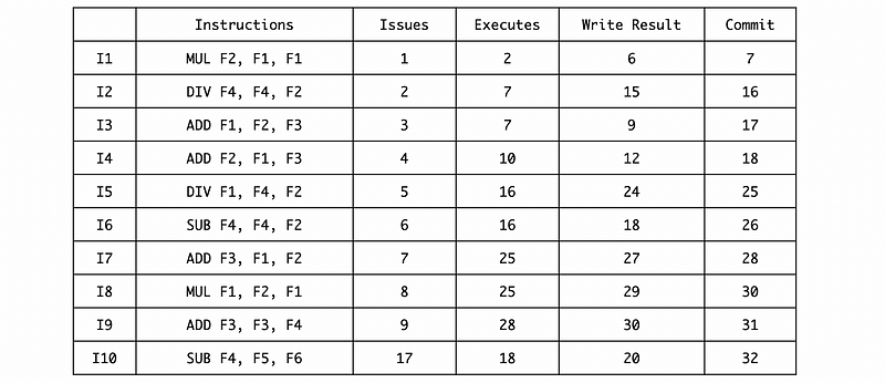
Example 4-3. (Exception and ROB) Suppose we have the following instruction sequence and registers values,
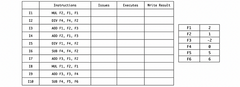
We have the following assumptions for executing this program,
- using Tomasulo’s algorithm
- multiplication takes 4 cycles for execution
- divide takes 8 cycles for execution
- other instructions take 2 cycles for execution
- results are written in the cycle after the execution
- dependent instruction can begin execution after the results are written
- 1 ALU for MUL/DIV, and 2 reservation stations for MUL/DIV
- 1 ALU for ADD/SUB, and 4 reservation stations for ADD/SUB
- More than 1 execute: older priority
- More than 1 write to the bus: ADD/SUB over MUL/DIV
- 1 ALU can execute only 1 instruction in a cycle (no ALU pipeline)
- only 1 instruction issuing per cycle
- only 1 CDB for writing results
a. Fill in the table with cycles.
b. Confirm that instruction I5 causes a divide-by-zero exception. Suppose this exception is detected at the very end of the 6th (6/8) cycle of the DIV execution stage. And nothing can be done about it until the start of the next cycle. If the exception handler prints out the values of F1, F2, F3, and F4, what will be these values?
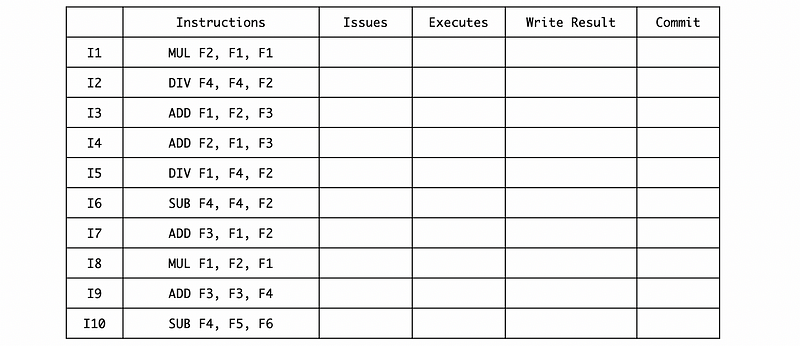
c. Suppose we add an 8-entry ROB to deal with this exception. Assume that no more than one instruction can be committed in each cycle and the instruction can only be committed in the cycle after writing the result. Remember that the RS is freed as soon as possible with a ROB. Fill in the following new table with cycles.
d. With the same assumption of question b but with this ROB, if the exception handler prints out the values of F1, F2, F3, and F4, what will be these values?
a. Ans:
First, we can issue the first 4 instructions and we have to wait for a MUL/DIV RS space for I5,
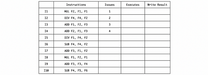
Then we can fill in the timing of these 4 instructions by the given information,

The next DIV can be issued in cycle 7 after instruction I1 writes the result and frees its RS, so
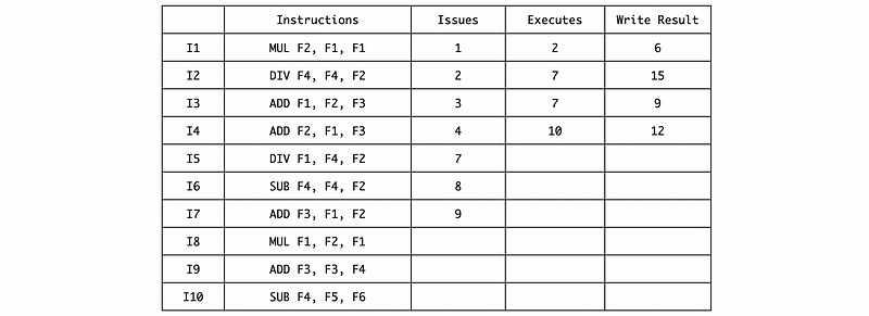
Because I5 and I6 are both RAW dependent on I2, so they need to be executed in cycle 16. And also the instruction I7 depends on I5, so it needs to be executed in cycle 25,
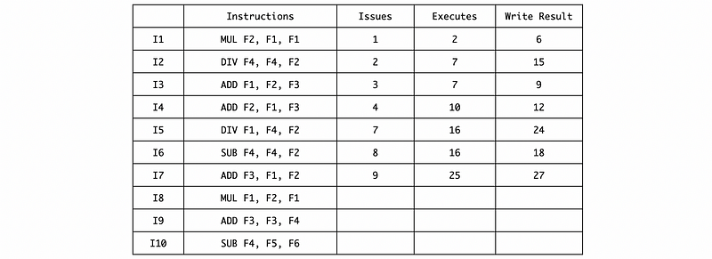
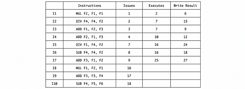
The instruction I8 should wait for the MUL/DIV RS space after writing the result of I2, so it has to be issued in cycle 16,
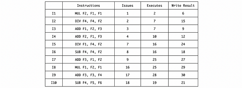
And the final timing result should be,
b. Ans:
Note that the execution stage for I5 takes 8 cycles and it starts from the 16th cycle. Thus, this exception is detected in cycle 22 (16+6) and we should call the exception handler in cycle 23.
As we can be confirmed from this timing table, because of the OOO execution, the instruction I6 and I10 is already written even it is not safe. Thus, although the exception is caused in the I5 when the program finally detects this exception, the F1 ~ F4 is not the result of the I1 ~ I4.
So, after I1 ~ I4, the registers should have,
F1           F2           F3           F4
-------      -------      -------      -------
2            0            -2           0
Note that we can confirm that there will be a divide-by-zero exception.
Then after I6, the registers should have,
F1           F2           F3           F4
-------      -------      -------      -------
2            0            -2           0
After I10, the registers should have,
F1           F2           F3           F4
-------      -------      -------      -------
2            0            -2           -1
c. Ans:
Note that I10 should be issued in cycle 17 because the ROB is full until cycle 17.
d. Ans:
The values of F1 to F4 will be,
F1           F2           F3           F4
-------      -------      -------      -------
2            0            -2           0
Example 4-4. (Register Renaming)
Given the following set of instructions, use register renaming to eliminate the false dependencies.
ADD R1, R2, R3
SUB R3, R2, R1
MUL R1, R2, R3
DIV R2, R1, R3
Assume there are 7 possible locations for the registers; L1, L2, L3, L4, L5, L6, L7. The registers at the start of the instructions are assigned as L1 = R1, L2 = R2, L3 = R3.
Ans:
R1 will be rewritten by the first instruction, so we have to eliminate the possible previous WAR dependency by renaming R1 to L4,
ADD L4, L2, L3
Continue and renaming the whole program,
ADD L4, L2, L3
SUB L5, L2, L4
MUL L6, L2, L5
DIV L7, L6, L5
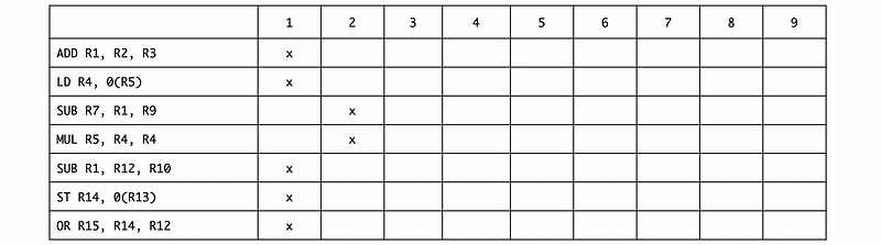
Example 4-5. (ideal processor IPC and ILP)
Suppose we have the following instructions,
ADD R1, R2, R3
LD  R4, 0(R5)
SUB R7, R1, R9
MUL R5, R4, R4
SUB R1, R12, R10
ST  R14, 0(R13)
OR  R15, R14, R12
Assume that the processor can execute in any order that doesn’t violate true dependencies (means that we can do the register renaming), and all the instructions have 1 cycle latencies (means that the whole any kinds of instruction will be finished in 1 cycle).
a. Suppose the processor’s ALU can execute any kinds of instructions in the fragment, and the processor can only execute up to two instructions in a cycle. Calculate the IPC.
b. Suppose the processor’s ALU can execute any kinds of instructions in the fragment, and the processor can execute up to four instructions in a cycle.
c. If we can not do the register renaming (means that we can not violate the data dependencies) based on some faults of the processor, with all the other features hold from question b. Note that the read and write to the same register can happen in one cycle. Will the IPC change? Explain why.
d. Calculate the ILP of this program.
a. Ans:
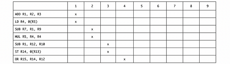
Based on this table, the IPC is 7/4 = 1.75.
b. Ans:
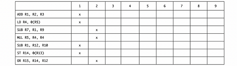
Based on this table, the IPC is 7/2 = 3.5.
Note that we can execute SUB R1, R12, R10 in the first cycle and then SUB R7, R1, R9 in the second cycle without worrying about the WAR dependency because we have the register renaming.
c. Ans:
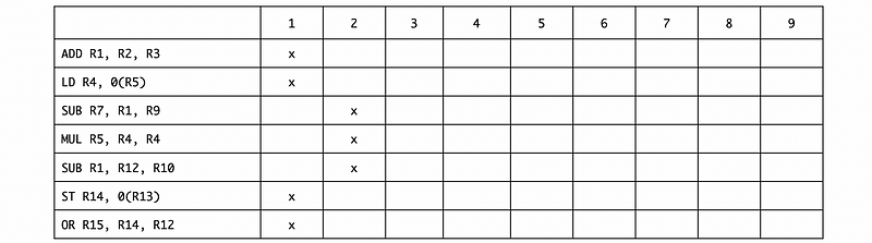
If we have to avoid all the data dependencies without register renaming, we need to execute SUB R1, R12, R10 in the second cycle. Based on this table, the IPC is 7/2 = 3.5. Because we still need 2 cycles to finish the execution, the IPC of this program won’t change.
d. Ans:
The ILP means an ideal processor that can do,
- the processor does the entire instruction (FDEMW) in 1 cycle
- the processor can do any number of instructions in the same cycle, but it still has to obey the true dependencies
So then, we are going to have,
We can find out that even we can execute 5 instructions in the first cycle, we still need to have the second cycle because of the data dependency. Based on this table, the ILP of this program is 7/2 = 3.5.
Example 4-6. (Tomasulo’s Algorithm)
Suppose we have a processor with dynamic scheduling with the following features,
- issue-bound fetch means that the operands are fetched during the instruction issuing
- RS is freed at the beginning of the writing stage
- an instruction can be executed in the cycle after its dependent instructions are written
- 1 ADD/SUB ALU, with 1 RS for this ALU
- 1 MUL/DIV ALU, with 1 RS for this ALU
- 1 LOAD/STORE ALU, with 1 RS for this ALU
- out-of-order issue (no need to follow the instruction queue)
- out-of-order execution
- no data forwarding
- Load/Store takes 2 cycles
- Add/Sub takes 1 cycle
- MUL takes 2 cycles
- DIV takes 4 cycles
Suppose we have the following instruction sequence. Fill in the timing table.
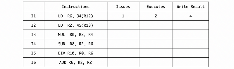
Ans:
We have to be careful about the out-of-order issuing, and this means that we can issue more than 1 instruction in the first cycle. The final result should be,

5. Memory Ordering, Compiler ILP, and VLIW
(1) Load-Store Queue (LSQ)
The load-store queue (LSQ) is the structure that stores the data needed to read/write from/to the memory at commit in order.
(2) Store-to-Load Forwarding
When a load command is put into the queue, the requested address of the load is compared to all previous store addresses in the queue. If there is a match, this value in the queue is used and eliminating the need to go to the memory.
(3) Missing Address Exception
It is possible that some store addresses are not ready (i.e. because of the cache miss) when the load instructions check the address for the load-to-store forwarding. The most common way to deal with this is to go to the memory and load the data anyway. If we read a stale value, we have to do a recovery.
(4) Compiler Technique #1: Tree Height Reduction
Tree height reduction is used for re-grouping an associative calculation to reduce the long dependency chain.
(5) Compiler Technique #2: Instruction Scheduling with Compiler
The compiler can reschedule the code to fill in the stalls caused by dependencies. This is called instruction scheduling.
(6) Compiler Technique #3: If-Conversion
If-conversion means to execute both ways of a branch and finally choose between them. It allows for greater flexibility in the instruction scheduling.
(7) Compiler Technique #4: Loop Unrolling
Loop unrolling creates a loop with fewer iterations by having each iteration do the work of two or more iterations.
(8) Compiler Technique #5: Function Inlining
Inlining involves removing the function call and replacing it with the body of the function.
(9) Superscalar
The superscalar processors are processors that can finish more than 1 instruction per cycle without long instruction words. The superscalar tries to FDEMW more than 1 instruction in each stage.
(10) VLIW
The very long instruction word (VLIW) processors load the commands into instruction words and split them if there are data dependencies. It may results in many NOPs in order to deal with the dependencies. This is especially useful for digital signal processing (DSP).
Example 5-1. (VLIW and Compiler ILP)
Suppose have a VLIW processor with 16 registers and the following units,
- A branch unit (for branch and jump operations), with a one-cycle latency
- A load/store (LW/SW operations) unit, with a six-cycle latency
- Two arithmetic units for all other operations, with a two-cycle latency
Each instruction specifies what each of these four units should be doing in each cycle. The processor does not check for dependencies nor does it stall to avoid violating program dependences the program must be written so that all dependencies are satisfied. For example, when a load-containing instruction is executed, the next five instructions cannot use that value.
If we execute the following loop (each row represents one VLIW instruction),
Loop:
    LW   R4, 0(R0)
    ADDI R0, R0, 4
    LW   R5, 0(R1)
    ADDI R1, R1, 4
    ADDI R2, R2, 4
    ADD  R6, R4, R5
    BNE  R2, R3, Loop
    SW   R6, -4(R2)
which performs element-wise addition of two 60-element vectors (whose address are in R0 in R1) into a third (address is in R2), where the end address of the result vector is in R3, and each element is a 32-bit integer:
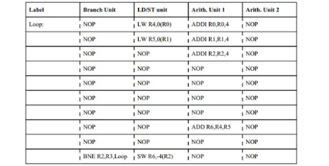
Note how we increment the vector points while waiting for loads to complete. Also, note how each operation reads its source registers in the first cycle of its execution, so we can modify source registers in subsequent cycles. Each operation also writes its result registers in the last cycle, so we can read the old value of the register until then. Overall, this code takes ten cycles per element, for a total of 600 cycles.
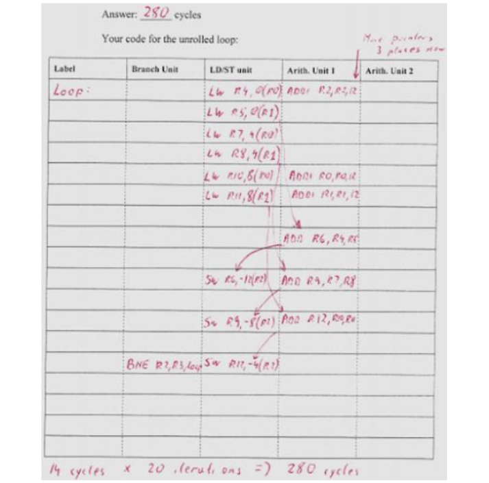
We will unroll (unroll twice) so three old iterations are now one iteration, and then have the compiler schedule the instructions in that (new) loop. What does the new code look like (use only as many instruction slots in the table below as you need) and how many cycles does the entire 60-iteration (20 iterations after unrolling) loop take now?
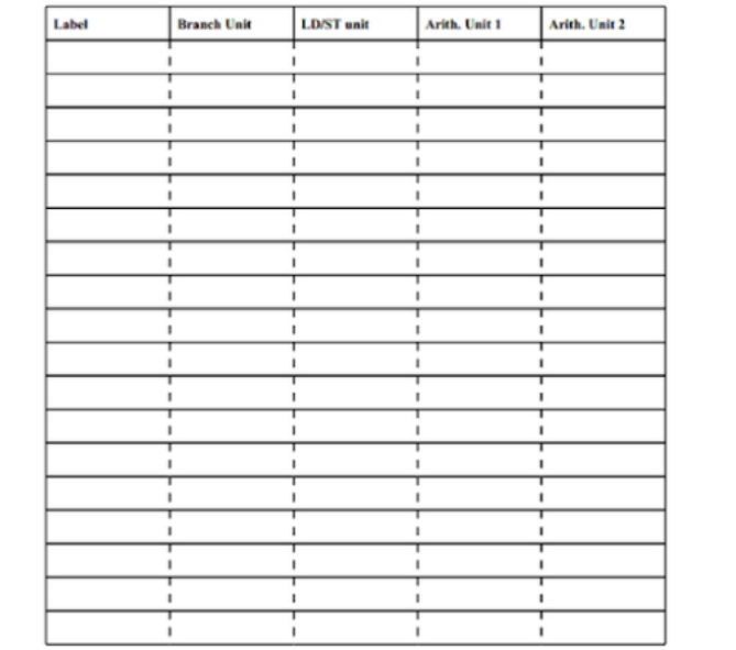
Ans:
The C code for this program is,
v = a + 60;
while (a != v) {
    c[i] = a[i] + b[i];
    i++;
}
If we unrolling twice, the C code should be,
v = a + 60;
while (a != v) {
    c[i] = a[i] + b[i];
    c[i+1] = a[i+1] + b[i+1];
    c[i+2] = a[i+2] + b[i+2];
    i += 3;
}
Then the assembly code should be,
Loop:
    LW   R4, 0(R0)
    ADDI R2, R2, 12
    LW   R5, 0(R1)
    LW   R7, 4(R0)
    LW   R8, 4(R1)
    ADDI R0, R0, 12
    ADDI R1, R1, 12
    LW   R10, 8(R0)
    LW   R11, 8(R1)
    ADD  R6, R4, R5
    SW   R6, -12(R2)
    ADD  R9, R7, R8
    SW   R9, -8(R2)
    ADD  R12, R10, R11
    BNE  R2, R3, Loop
    SW   R12, -4(R2)
We can write the result in the table as,