High-Performance Computer Architecture 22 | Locality Principle, Cache, Types of Caches, LRU, and…
High-Performance Computer Architecture 22 | Locality Principle, Cache, Types of Caches, LRU, and Write Policies
- Locality Principle
(1) The Definition of Locality Principle
Things that will happen soon are likely to be close to things that just happened. Based on this principle, we have already used this principle for branch prediction, and now, it is time to be used for caches
(2) Locality Principle: Memory References
If we know that the processor has accessed an address recently, the locality principle says that,
- the processor is likely to access the same address again in the near future
- the processor is likely to access addresses close to this address
(3) The Definition of Temporal Locality
Temporal locality means that once we access an address, we are likely to access the same address again. In the example above, the processor is likely to access the same address again in the near future is actually a temporal locality.
(4) The Definition of Spatial Locality
Spatial locality means that if we access an address, we are likely to access nearby addresses so on. In the example above, the processor is likely to access addresses close to this address is actually a spatial locality.
(5) Locality Example: Finding Information
Suppose we would like to find the information from the library, and you can imagine that the library is quite large, so it will be quite slow for us to find the book we need if we do a one-by-one search.
If every time we go to the library, we would like to find a book about the locality principle, we will end up searching at the same place. This happens to be a temporal locality.
However, we may also want to search for some books about computer architecture. So what we can do is to find the books close to the books about the locality principle. And this is what we called a spatial locality.
So now, a student will have three options on that,
- Go to the library, find the info, go back home
- Go to the library, borrow the book, go back home
- Go to the library, borrow all the books we may need in the future, and build a smaller library at home
The first option is quite time-consuming and we do not benefit from the locality. The second option is reasonable because it does exploit temporal locality and spatial locality, and we eliminate the time we need for searching the same thing many times. This is why most people choose this option. Although the third option saves our future time on the trip, it is very expensive for us. What’s more, we also have to search among many books, finding them on the shelves and so on.
(6) From Locality to Cache
Like in the library example, we would like to borrow some books we need and close to us, but we won’t borrow too many books because this can also be slow and expensive.
So for the computer architecture, we would like to have a small amount of data compared to the memory, but it should keep the information that we are really interested in. So that small repository of information is called a cache when we are talking about memory accesses.
2. Cache
(1) The Definition of Cache
The cache is a small memory inside a processor where we are trying to find the data before we go to the main memory.
(2) The Properties of Cache
Let’s now take some time to think about what we need for a cache,
- Fast: means that the cache has to be small
- Not everything will fit: this is because the cache is small
- Access states: it is possible that the data we want is in/not in the cache, so this brings us to two different access states
(3) Two States for Cache
Basically, we have two states for each cache,
- Cache Hit (Hot Cache): This means that the data we want to access is already in the cache (quick)
- Cache Miss (Cold Cache): This means that the data we want to access is not in the cache (slow)
When we have a cache miss, we will copy this location to the cache so that the next time we access it, we will hopefully benefit from the locality and have a cache hit. Based on the locality principle, we can know that the cache miss happens rarely and it is reasonable for us to design caches.
(4) Cache Performance
There are several metrics that can be used to measure the performance of a cache,
- Average Memory Access Time (AMAT): the access time to memory as seen by the processor. AMAT can be calculated by,

The lower the AMAT, the better the cache. To lower the AMAT, we have to reduce the hit time (by using a small & fast cache), reduce the miss rate (by using large and/or smart cache).
The miss penalty is also called the main memory access time (MMAT), which can be very large compared with the hit time.
Thus, if we want to improve the performance of our cache, we have to make a balance between the hit time and the miss rate. Although some caches can be extremely small and fast, we have to pay the cost of a high miss rate because of cache misses.
- Miss Time: the miss time means the overall time it takes if we have a cache miss and it is defined by,

Miss time is also the time we have to pay for a cache miss.
(5) General AMAT
Based on the previous average memory access time (AMAT) definition and the miss time we have already talked about, we can have the following expression as a general AMAT expression,

(6) Cache Size
We have seen that we want to keep our cache small and fast, but we also have to keep in mind that the cache can not be too small because then it keeps very little stuff. However, in the real processors, we do not have only one cache. The cache that directly services the read/write requests from the processor is always called an L1 cache or a level-1 cache. This is what we are going to discuss for its size.
By the way, it can be quite complicated if we have a cache miss in the L1 cache, and then instead of going directly to the main memory, we will go to some other caches. We are going to talk about this later.
So how big is the L1 cache? In recent processors, the typical size of the L1 cache has been 16 KB to 64 KB, and this is large enough to get about a 90% hit rate. Moreover, it is also smaller enough to have a hit time of only 1~3 cycles.
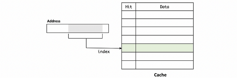
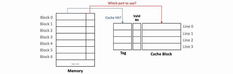
(7) Cache Organization
Let’s discuss how the cache is organized so as to determine whether we have a cache hit or a cache miss. Conceptually, the cache can be treated as a table with some bits that we take from the others of the data. In each line/entry of a cache, some bits are going to tell us whether we have a hit or not, and there are also some other bits that are really the data we want if we do have this data in the cache. The cache will be indexed with some bits that we have taken from the address of the data.
(8) Cache Block Size
How much data we have in each entry is called the block size (aka. line size) because each entry in the cache is also called a block (aka. line). The block size is defined as the number of bytes are in each of these entries.
Imagine a situation that we have a block size of 1 byte. This means that the data that can be stored in each of the entries is 1 byte. Even though this works for most of the immediate values, we have to notice that for some load/store operations, what we want to look up in the cache are addresses that will take up 4 bytes each. Thus, one entry won’t be enough to store this data and we should look up 4 different lines in the cache. So the block size won’t be that small.
Imagine another situation that we have 1 kb as the block size. In this case, we will fetch a lot of data from the memory every time when we have a miss. As a result, if there is not enough locality, a lot of data will not be used. So we are occupying spaces in our cache. Remember that the modern caches have only 16~64 kb, so this block will also consuming a significant part of the cache and much of the data that we are passing is not going to be used in the future.
Therefore, for the L1 cache, we don’t want the block size to become too large (like 1 kb), and we also don’t want the block size to become over small (like 1 byte). So block size of 32 bytes to 128 bytes are made for the modern caches because we balance between the use of spatial locality, and not depend too much on the spatial locality since most programs don’t have that much.
(9) Aligned Block Starting Address
For all reasonable caches, we will only consider aligned blocks which means that we can not fetch any 64-byte blocks from the memory to the cache. Instead, we need to fetch the 64-byte block that contains the data and has its block aligned. Let’s see why.
Suppose we have a block starting address that starts from anywhere in the memory. Thus, in the cache, we may probably have the first entry ranges from address 0~63, and the second one ranges from 1~64. Because the blocks are not aligned, you may find these two entries have an overlapped part from the address 1~63, and this can be useless.
The term aligned means that the blocks should not have data that overlap with each other. For example, if the first entry ranges from 0 to 63, then the second one should be 64~127.

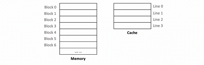
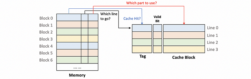
(10) From Memory to Cache
Now, let’s see how can the data in the memory be fetched into the cache. Suppose we have a computer that each address has 1 byte, and we also have a cache whose cache block size is 16 bytes. Then, 16 addresses in the memory will be combined as a block (e.g. block 1 and block 2 in the following diagram), and then the data will be fetched in a line of the cache.
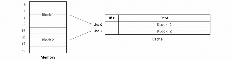
Note that we can always confirm that the block size is always equal to the line size.
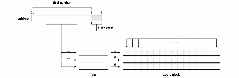
(11) Block Offset
Suppose we have a cache with a block size of 16 bytes (thus we need at least 4 bit to index these 16 bytes), then as we have discussed above, 16 addresses in the memory will be mapped to the same block. When the processor wants to get the data, it will produce a 32-bit address, which represents the location that the processor wants to find in the cache. The 0 to 3 bits of this address tell us which part of this block should we read and the remaining bits (4 to 31) tells us which block we are trying to find.
The bits that tell us where in the block are we going to find the data are called the block offset and the bits that tell us which block are we interested in are called the block number.

So what we do is that,
- access the cache
- find the block we need according to the block number
- get the right data from the block by the block offset
(12) Block Offset: Example
Suppose we have a cache that has a block size of 32 bytes, and we have a 16-bit address used to lookup data from this cache,
1111 0000 1010 0101
Then the block number should be,
1111 0000 101
The block offset should be,
0 0101
This is because we need at least 5 bits for indexing a 32-byte cache block.
(13) Cache Tags
We have known that the processor can use the block number to find which block to access. So how does this implement? The answer is by using tags. The tags can be treated as the unique ID of the blocks in the cache. If the block number equal to the tag for a block, then we can confirm that we have a cache hit, and then the block offset can be used to find which data to use.
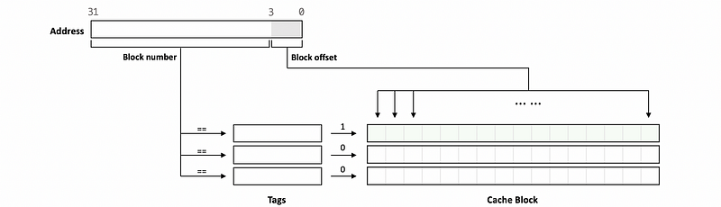
Note that the tags can be part of the block number, and this means that the block number doesn’t have to be equivalent to the tag. So in a more general case, we might have the following diagram,
(14) Valid Bit
Let’s think about the following situation. Suppose we have initialized a program, and after that, all the tags and cache blocks contain some garbage values. If we have a tag with its initial value as,
00 0000
And there is a block number that contains this tag, and the part of it used for indexing is also this. Then, the processor will mistakenly think that we have a cache hit and starts to read some garbage values from the corresponding cache block.
In order to deal with this problem, what we do is to add an additional bit of state to the cache. So before we check the equality of the block number and the tag, we have to check for the valid bit. Initially, all the valid bits will be set to 0, and this means that even though the block number is equal to the tag, it will not be a cache hit.
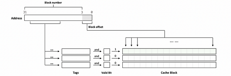
This is to say that, generally, the hit condition should be,

3. Types of Caches
(1) Three Different Types of Caches
Basically, we have three types of caches,
- Fully Associative Cache: any block from the memory can be put into any line of the cache. Thus, if we have 16 lines in the cache, we have to search up to 16 lines in order to find the block we are looking for.
- Set Associative Cache: a block from the memory can only be put into N lines (where N can be 2~8). So if we want to find a block, we only need to search for these N lines.
- Directed Mapped Cache: a block can only go into 1 line of the cache. Thus, we only need to check one line in the cache.
Now, let’s talk more about these different types of caches.
(2) Directed Mapped Cache
Suppose we have the following memory and a 4-line cache,
Suppose we have the following mapping rules,
Block 0 -> Line 0
Block 1 -> Line 1
Block 2 -> Line 2
Block 3 -> Line 3
Block 4 -> Line 0
Block 5 -> Line 1
Block 6 -> Line 2
Thus, we have,
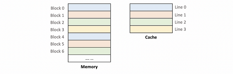
We can conclude that each of the blocks in the memory can only go to only 1 specific line in the cache. So this cache is a direct-mapped cache. Then, let’s take a careful look at the block memory address.

- Block offset: decides which part of the data we will use in the cache block
- Index: decides which line of the cache should we go to. Because we have 4 lines in the cache, a 2-bit index is enough for indexing.
Index
00      ->     Line 0
01      ->     Line 1
10      ->     Line 2
11      ->     Line 3
- Tag: Even though each of the memory blocks can only be mapped to 1 line of the cache, a line can have many blocks mapping to it. For example, both
Block 0andBlock 4will be mapped toLine 0. Thus, we have to decide what is really in the cache,Block 0orBlock 4. Because both ofBlock 0andBlock 4have the same index of00, the index bits are not useful for identifying these blocks. However, the rest of the block numbers can be treated as an ID to trace these different blocks. Therefore, these bits can be treated as tags and used to decide if we have a cache hit.
So in general, the final diagram could be,
(3) Evaluation of the Direct Mapped Cache
let’s now look at the upsides and the downsides of the direct-mapped cache. The upsides are,
- Fast: because we only have to check for 1 line in the cache for each block
- Cheaper: because we only have to do 1 comparison of the tag and the block number
- Energy Efficient
The downsides are,
- Conflict: when we have a block B that has the same index of block A in the cache, block A will be kicked out even if it can be useful in the cache. This brings us to the result that different blocks will fight to the 1 line in the cache.
- Higher Miss Rate: the more conflicts, the higher the miss rate.
In conclusion, although the direct-mapped cache can benefit from fast access, it should pay a higher miss rate because of the conflicts.
(4) Direct Mapped Cache: An Example
Suppose we have a 16 kB directed-mapped cache, 256-byte blocks which of these conflict with 0x12345678, then,
- the block offset of this address should be the 8 (because
log2(256) = 8) least significant bits0111 1000 - the index of this address should be 6 bits long (because
log2(16*1024/256) = log2(64) = 6). And the index should be01 0110 - The rest of the address will be the tag, which should be 18 bits.
- the address
0x12345677will not cause a conflict because it is in the same block of the original address - the address
0x12341666will cause a conflict because they will be mapped into the same line but the tag of them are not the same
(5) Set Associative Cache
In a direct-mapped cache, the index is used for getting the right line. While in a set-associative cache, the index is used for directing to the set, and the set is defined as a combination of several lines. An N-way set-associative cache means that each of the sets in the cache has N lines. So for a given block in the memory, it can be mapped to N possible lines in a set.
Suppose we have a two-way set-associative cache and each of the sets in this cache has 2 lines, so a given block can be in either of these two lines. In the following diagram, we have a 4-line 2-set two-way set-associative cache,
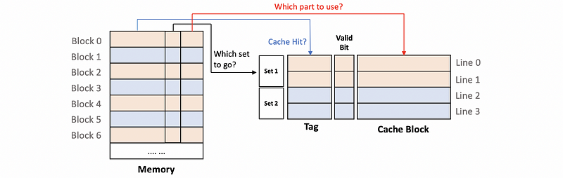
The upsides of the set-associative cache are,
- Reduce the conflicts: the conflicts can be reduced because now we can have several lines for storing the same block
- Reduce the miss rate: because we have reduced the conflicts in the cache, there is a trend that we can have a higher miss rate
The downsides of it should be,
- Slow: because we have to search up to N times in the set to decide whether there is a cache hit
(6) Fully Associative Cache
A fully associative cache is a cache that any memory blocks can be mapped to any lines in the cache. This means that we do not have to use the index anymore. So all the remaining bits in the address will be considered as the tag.
(7) Relationship of Three Types of Caches
The direct-mapped cache and the fully associative cache are actually two specific cases for the set-associative cache. If we have a 1-way set-associative cache, then this will be equivalent to a direct-mapped cache. Meanwhile, if we have a fully-associative cache, then this means that have a #-of-lines-way set-associative cache. Thus, for all these three types,
- Offset Size = log2(block size)
- Index Size = log2(# of sets)
- Tag Size = the size of the remaining bits
4. Cache Replacement
(1) The Definition of Cache Replacement
We have discussed how cache finds the data when we are looking for it. Now let’s talk about what happens when we need to remove something from the cache to make room for the other data. When the set for a memory block is full but we also have a cache miss problem, we have to do cache replacement.
(2) Common Cache Replacement Algorithms
To decide which block should we kick out, normally we would have the following policies,
- Random
- FIFO
- Least Recently Used (LRU): LRU is a good policy but it is not easy to do
- Not Most Recently Used (NMRU): a policy to mimic the LRU
(3) Implementing LRU
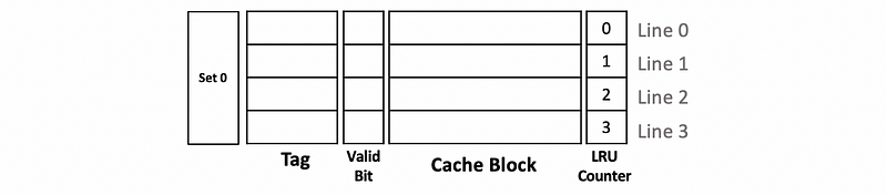
Now let’s see how we can implement the LRU. Suppose we have a 4-way associative cache and let’s track what’s happening in a single set. Continue to what we have discussed, this set should be as follows,

Now because we want to know which block is the least recently used one, we will add the LRU counters to each of these blocks.
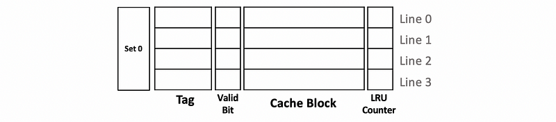
The values in the LRU counter should all be different all the time. So initially, the value will be set to 0 (means least recently used) to 3 (means most recently used) according to the size of the set (i.e. in this case, 4). Thus, we have,
Now assume that we have a cache replacement and the LRU block according to the set is line 0. So we will kick the data in line 0 out and then update the LRU counter. Because now the line 0 is just used recently, it becomes the most recently used and the LRU counter should be set to 3. Because we have discussed that the LRU counters should all be different in a set at any time, we should also update the values in other counters by decreasing 1.

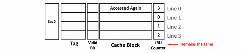
If line 0 is accessed again, then line 0 will still be the most recently used block and the LRU counter should not change.
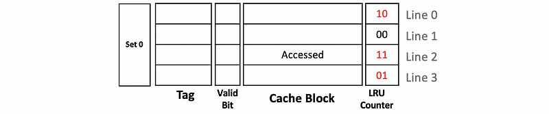
If now the block in line 2 is accessed, then we can conclude that the block in line 2 should be the most recently used block. So we have to update the value of the LRU counter to 3 for line 2. Instead of decreasing all the other LRU counters by 1, in this case, we will only reduce 1 to the LRU counter that is larger than the original value of the LRU counter in line 2 (i.e. 1) and these counters are the LRU counter for line 0 and line 3. For those whose values are below the original value of the LRU counter in line 2 (i.e. the value of line 1), we will keep its value. By doing so, we will maintain that all the LRU counters are different all the time.

Note that after each step, we can check that all the LRU counters in a set have different values. If some of the counters have the same value, we might probably make some mistakes somewhere.
(4) LRU Cost
We have to take care of the cost of the LRU. In the example above, we have a 4-way set-associative cache, and each of the LRU counters needs to have 2 bits if we want to express value 0~3. So in reality, the final state that we have discussed should be,
Therefore, generally, if we have an N-way set-associative cache, we will need log2(N) bits for each counter.
If the value of N is higher, like 32, then we need to have 5 bits in each counter and the cost of maintaining these LRU counters can be really high. Also, because we have to update 32 5-bit counters on each access even for the cache hits, the LRU can be very energy-consuming.
To deal with the LRU cost, the LRU approximations like NMRU try to keep fewer counters and fewer updates on cache hits.
5. Cache Write
(1) Cache Writing Policy
We have already discussed the read policy for a cache, and now, let’s discuss what if we write to the cache. Normally, we are concerned about two different aspects when we write to the cache,
- Do we insert the block we write to the cache?
- Do we also update the memory?
(2) Types of Caches: Part 1
When we write to the cache if we have a write miss, should the block brought to the cache or not? There are two types of caches,
- Write-allocate Cache: bring the write miss block to the cache
- Non-write-allocate Cache: not bring the write miss block to the cache
Most caches today are write-allocated caches because there is some locality between reads and writes. This means that if we write to something, we are also likely to read from it.
(3) Types of Caches: Part 2
The other aspect of the writing policy is that when we have a write, should we write only to the cache, or should we also write to the memory immediately? There are also two types of caches based on this policy,
- Write-through Cache: This means that we will update the memory immediately
- Write-back Cache: under this policy, we first write to the cache, and then we write to the memory when the block is replaced from the cache
Write-through caches are quite unpopular because they send stuff to memory directly. We usually want to have a write-back cache because it prevents the memory from being overwhelmed and reduces the number of writes that we might have.
(4) Relationship between Write-allocate Cache and Write-back Cache
If we want to have a write-back cache, we also need to have it as the write-allocate cache. This is because the write-back cache must have the write block in the cache so that we don’t need to update it in the memory.
(5) Write-Back Cache Problem: Distinguish Between Read/Write
However, if we want to implement a write-back cache, there can be a tricky problem. Some blocks in the cache will be the blocks that we have read from the memory, and the other blocks will be the written ones. For the read blocks, we don’t have to update the memory if we kick them out of the cache, while for the written block, we have to write them to the memory if they expire from the cache. So the problem is that how can the processor know whether a block is read or written?
Probably, we have the following options,
- Write All: Regardless of whether it is a read block or a written block, we will write to the memory every time we replace a block. The problem is that we can have many read stuff and this will end up writing to memory over and over again.
- Dirty Bit: As another option, we can add a dirty bit to every block in the cache. The dirty bit shows whether we have written the block since it was placed in the cache or not. If the dirty bit equals 0, it means the block is clean and this block is not written since it was last brought from the memory. If the dirty equals 1, it means the block is dirty and we should write this block back to the memory when a replacement happens.
(6) Write-Back Cache: An Example
Again, we will use an empty 4-way set-associative write-back cache with dirty bits in this case. We will only talk about set 0 of this cache. Thus, initially, we can have,

Suppose we have the following operations,
WR A
RD A
RD B
RD C
WR C
Let’s see what will happen when we conduct these operations.
When we have the first write to A, because this is a written block, the dirty will be set to 1.

Then when we read from A, the processor checks the tag and the valid and determines that we have a cache hit. So A will be directly read from the cache.

Then we read B and we can find that B is not in the cache (cache miss). Thus, B will be read into the cache, and the dirty bit of B will be set to 0.

Also, when we read C, we have a cache miss. C will be read into the cache, and the dirty bit of C will be set to 0.

Finally, because we write to the C, the processor checks the cache and finds a cache hit. So we update the cache block and set the dirty bit to 1. Because our cache is a write-back cache, we don’t have to update the memory now.