High-Performance Computer Architecture 23 | Virtual Memory, Virtual to Physical Translation, Page…
High-Performance Computer Architecture 23 | Virtual Memory, Virtual to Physical Translation, Page Table, and Translation Look-Aside Buffer
- Virtual Memory
(1) Processor’s View of Memory
The processor sees what we called the physical memory, which is the memory contained in the actual memory modules that we bought and put on the system.

The amount of the memory sometimes is even lower than 4 GB and it is almost never 4 GB per process we have in the system because we can have tens or hundreds of processes. Even though the memory address is 64 bits, which can be mapped to at most 16 EB per process, we will never have that much memory.
So the amount of physical memory we have is usually less than what all the programs can access. Actually, the addresses the processor uses for the physical memory have a 1:1 mapping to the bytes or words in the physical memory. Thus, a given address always goes to the same physical location and a physical location always has exactly one physical address.
(2) Program’s View of Memory
The program usually sees a huge amount of memory and some continuous memory regions are actually used by the program. But there’s also an enormous region in the middle between the stack and the heap that the program will never access unless the stack and the heap keep growing. However, the heap is relatively small compared to how much space we have here because it’s a huge amount of memory.
As a result, although the program thinks that it has a lot of memory, what it really accesses when executing is actually a relatively small proportion.
(3) The Definition of Virtual Memory
We have discussed that the program thinks that it virtually has a lot of memory, but in practice, there isn’t that much memory. Thus, this technique to deceive the programs is called virtual memory.
(4) Virtual to Physical Mapping
When a program generates a virtual address, the processor needs to access some physical address. So how does the processor map what the program is trying to access to what the processor should be accessed?
The simplest idea is to build a large table that contains all the mapping rules for each program. However, we will not implement this in practice because these tables would consume a lot of our memory and it is quite hard to search a rule in a table.
A more advanced idea is to divide that virtual memory into small blocks (called pages) so that we can reduce the size of the mapping table. In addition, the physical memory will also be divided to small blocks (called frames) in order to adapt to the pages. Commonly, the size of a page/frame is 4 kB and the OS decides how to do the mapping.
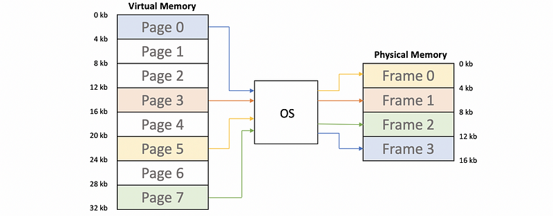
Note that the actual mapping mechanism is called a page table that says for each page of a process, which frame will it be mapped in the physical memory.
(5) Location of the Missing Memory
In the example above, we can find out there are 4 pages being mapped to the physical memory. But where are the rest of these pages? The answer to this problem is that these pages are on the hard disk.
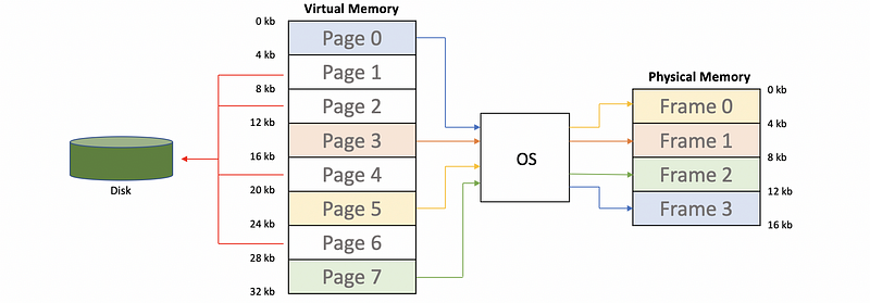
Because these pages are store in the disk, they can not be directly accessed by the processor and the processor can only load/store from the physical memory.
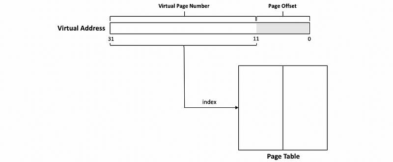
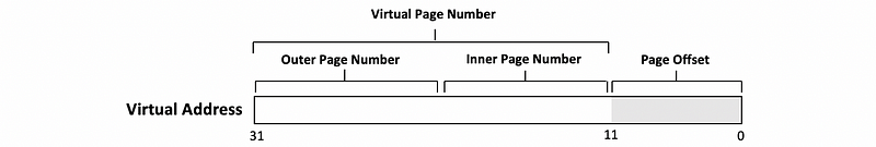
(6) Virtual Address
Similar to the cache memory, the virtual can be divided into two parts. Some least significant digits are called the page offset, which is used to identify which data we need in a frame of the physical memory. If we have a page size of 4 kB (i.e. 4*1024 Bytes), then the size of a page offset is 12 bits (because log2(4*1024) = 12).
The rest of the virtual address is called the virtual page number.

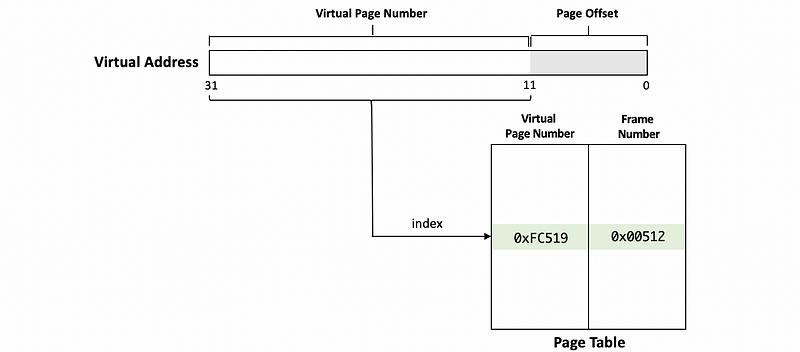
(7) Virtual Address: An Example
Now, let’s see an example about the virtual address. Suppose we have a 32-bit virtual address and the page size is 4 kB,
0xFC51908B
Then the least significant 12 bits are telling us the page offset, which should be,
0x08B
The rest of this address is called the virtual page number,
0xFC519
Now, we will use this value to index into the page table. In this case, the index into the page table will be 0xFC519 and we will find an entry corresponding to this index in the page table.
(8) Page Table
The page table tells us what the frame number corresponds to the given virtual page number.

So generally, now the diagram will become,
(9) Virtual to Physical Address Translation
Now that we have the corresponding frame number based on our virtual page number, and what we need to do now is to generate the physical address that we need. This operation is called a virtual to physical address translation.
After we retrieve the physical frame number from the page table, the page offset and the physical frame number will be put together to generate the physical address. Then this physical address is what we use to actually access the physical memory.
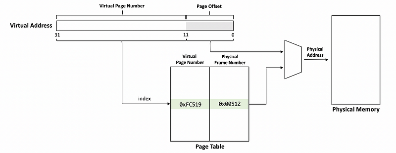
In our example above, the physical address would be,
0x0051208B
Note that the page offset is present in both the virtual and physical address, so during the virtual to physical address translation, the least significant bits of the virtual address does not change.
(10) Virtual to Physical Address Translation: An Example
Now, let’s see an example of the virtual to physical address translation. Suppose we have a 4-entry page table as follows,
Page Table
-------------
0x1F
0x3F
0x23
0x17
Also, the virtual address takes 16 bits, and the physical address takes 20 bits. And let’s translate the following virtual addresses to the physical addresses,
0xF0F0
0x001F
Because we only have 4 entries in the page table, the size of the virtual page number that we will use for indexing the page table will be 2 bits. Then because the virtual address takes 16 bits, the page offset takes 14 bits. The binary forms of these virtual addresses are,
1111 0000 1111 0000
0000 0000 0001 1111
The offset will not be changed and we grab the corresponding physical frame number based on the page table. So the physical frame number we are going to have, are
Index   Frame Number   Binary
-----   ------------   ------------
11      0x17           0001 0111
00      0x1F           0001 1111
Then we replace the virtual page number with the physical frame number (note that we should keep the offsets), so,
0001 0111 11 0000 1111 0000
0001 1111 00 0000 0001 1111
Reorganize these two addresses, we will have,
00 0101 1111 0000 1111 0000
00 0111 1100 0000 0001 1111
Because each physical address takes 20 bits, we can remove the most significant 2 bits because they are 0s. So the physical addresses are,
0101 1111 0000 1111 0000
0111 1100 0000 0001 1111
This is also,
0x5F010
0x7C01F
2. Page Table Optimization
(1) The Definition of the Flat Page Table
What we have discussed is so-called the flat page table where for every page number, there is an entry corresponding to it.
(2) Size of Flat Page Table
Based on the definition of the flat page table, we can know that,
- 1 entry (of the page table) per page (in the virtual address space)
An entry in the page table contains frame numbers and a few bits (e.g. the protection bits) that can be used to tell us if the page is accessible. So even though some pages in the page table are never accessed, the table keeps them, and thus the table can become unnecessarily large.
The size of a flat page table can be calculated as,

Because the number of the entries equals the number of the pages, the expression can be written as,

Imagine that we have a virtual memory of 4 GB and each page has a size of 4 KB. Also, the size per entry is 4 bytes. Then we can calculate the page table size for this virtual address space as,
PT_size = 4GB/4KB * 4B = 1024*1024*4 = 2^22 Bytes = 4 MB
(3) Flat Page Table Evaluation
If we have a large virtual address space, the size of a flat page table can be enormous. For example, the modern addresses will be 64 bits and if the application thinks that it can use all these memories, the size of address space it would have should be 2^64 bytes. Then for a 4 KB per page and 4 B per entry table, the page table size would be,
PT_size = 2^64B/4KB * 4B = 2^14 TB = 16 PB
For modern computers, this can be impossible because we can not have a memory of 16 petabytes. So the main problem with the flat page table is the size of it.
(4) Multi-Level Page Tables Idea
We have seen that the flat page table can be quite large even for 32-bit addresses, and it will be nearly impossible to implement for 64-bit addresses. Let’s see the multi-level page table that answers how we reduce the size of the page table when we have a large address space.
Let’s first recall the structure of virtual memory space. Suppose we have a 64-bit system (means that all the virtual addresses are 64 bits), then the virtual memory space should be,
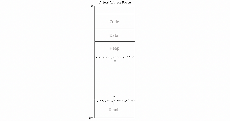
At the beginning of the virtual memory, there is the code, the static variables (data), and the heap that grows to the top. At the top of the virtual address space, there is the stack that grows to the bottom. So what is actually useful for us are two contiguous regions of virtual memory that actually used by the application.
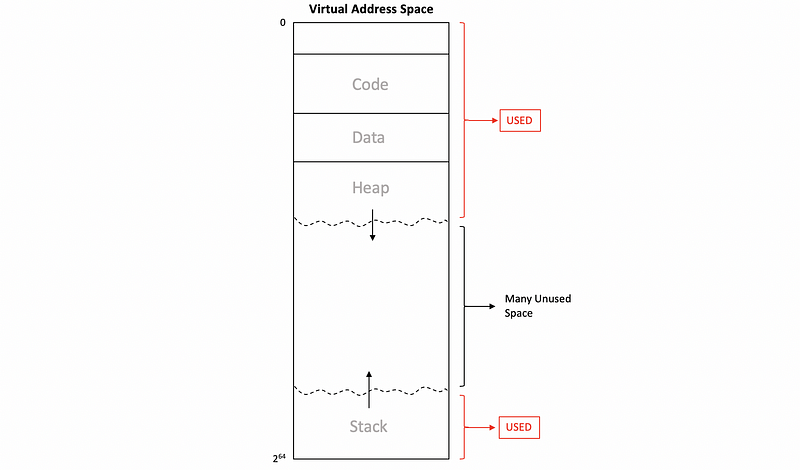
For a multi-level page table, even though we will also use some bits of the virtual addresses for indexing, we want to avoid the use of the table entries that correspond to the huge unused space. So the basic idea is to try to omit the unused space in the virtual space.
(5) Two-Level Page Table Implementation
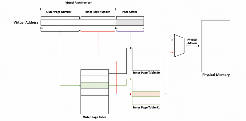
The virtual memory also consists of the virtual page number and the page offset. The difference is that the virtual page number will be divided into the outer page number (more significant bits) and the inner page number (less significant bits). These two numbers will index to different tables.
In the previous example, the outer page number tells us which part of the large page table we will be using and the inner page number tells us which specific entry in that large page table we would be using.
However, instead of having a large page table, the outer page number is now used to index into the outer page table. And each entry in the outer page table tells us which inner page table do we need to find. The inner page number is then used to index into the inner page table and what we can find there is the actual frame number to access.
(6) Two-Level Page Table: An Example
Now, let’s see a really simple example of the two-level page table. Suppose we have a virtual address with 8 bits. The least significant 4 bits are the offset and the most significant 4 bits are the page number (with a 2-bit outer page number and a 2-bit inner page number).
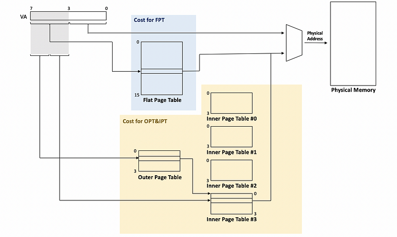
In this case, the cost for a flat page table is 16 entries, while the cost for the outer page table and inner page tables is 20 entries (i.e. 5*4 = 20 entries). We can observe that the implementation has an even higher cost compared with the flat page table. So where are the savings?
The saving is that if there is an unused large part of the address space (e.g. like the unused space between the heap and stack), the corresponding part in the outer page table will be marked as unnecessary, and the corresponding inner page table will be eliminated. For example,
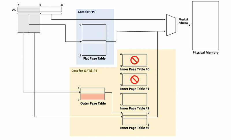
And now, the cost for all the outer/inner page tables will be 12 entries (i.e. 3*4 = 12). In a larger address space, the outer page table will have many pointers and most of these pointers will point to an unused inner page table. So we can simply eliminate these pointers from the outer page table.
(7) Size of Two-Level Page Table
Now, let’s discuss a real case about the size of a two-level page table. Suppose we have a 32-bit address space with a page size of 4 KB. Each of the outer page table and the inner page tables will have 1024 entries, and each entry takes 8 bytes.
Assume that we have a program that uses the virtual memory from 0x0 to 0x1000 and from 0xffff0000 to 0xffffffff. Calculate the size of a flat page table and the size of a two-level page table.
According to the definition of a flat page table, each of the addresses will be mapped to an entry. So the flat page table size will be 8 MB (i.e. 2³²/2¹² * 8 = 8 MB).
For the two-level page table, because the outer page table and the inner page tables each have 1024 entries, so both the outer page number and the inner page number are 10 bits long. Because the virtual address is 32 bits, then the offset is 12 bits (i.e. 32 - 10 - 10 = 12). So for the virtual addresses,
No    VA              Offset      Inner             Outer
---   -----------     -------     -------------     -------------
VA1   0x00000000      0x000       00 0000 0000      0000 0000 00
VA2   0x00001000      0x000       00 0000 0001      0000 0000 00
VA3   0xffff0000      0x000       11 1111 0000      1111 1111 11
VA4   0xffffffff      0xfff       11 1111 1111      1111 1111 11
We can find out that the VA1 and VA2 have the same outer page number and the VA3 and VA4 have the same outer page number. Thus, VA1 and VA2 will be mapped to the same inner page table (№ 0), while VA3 and VA4 will also be mapped to the same inner page table (№ 1023). Because all the other memories are not used by the program, we will not assign inner page tables to the corresponding pointers.
Thus, for this two-level page table, we have used 1 outer page table and 2 inner page tables. So the overall cost is 24 KB (i.e. 3*1024*8 = 24 KB), and we can observe a huge saving compared with the flat page table.
(8) Size of Four-Level Page Table
In the case above, we have discussed how to calculate the size of a 2LPT. Now let’s see how we can calculate the size of a 4LPT. Suppose we have a 64-bit virtual address space with 64 KB per page. The size of an entry in the page table is 8 bytes, and the program only uses the addresses from 0 to 4GB.
Assume we have a 4LPT with the page number split equally, then calculate the size of this 4LP table.
In this case, we can know that the offset should be 16 bits (i.e. log2(64*1024) = 16), and because the page number is split equally, they should have 12 bits each (i.e. (64 - 16)/3 = 12). So for the beginning VA to the ending VA, we will then have,
VA         0x0000 0000 0000 0000       0x0000 0001 0000 0000
------     ---------------------       ----------------------
Offset     0x0000                      0x0000
Outer1     0x000                       0x000
Outer2     0x000                       0x000
Outer3     0x000                       0x010
Inner      0x000                       0x000
Based on this table, we can know that all the pages we need will be on the same outer page table 1, the same outer page table 2, and the same outer page table 3. But they will be in the different inner page tables. The outer 3 have a range from 0x000 to 0x010, which contains 16 inner page tables in this range. Thus, we can have the following diagram,
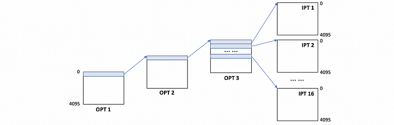
As a result, in total, we will have 19 tables (i.e. 3 outers and 16 inners) and each of them has 4096 entries (i.e. 2¹²). Because we have known that each entry takes 8 bytes, the overall size of this 4LPT will be 608 KB (i.e. 19* 4096*8 B = 608 KB).
(9) Page Size: Large or Small
We have known that the page size decides how many addresses we can have on a page. When we have a large page size, we will have more bits for page offsets. When we have a smaller page size, we will have fewer bits for page offsets. So should we have a large page size or a small page size? Here are some concerns,
- Size of page table
Because when we have a smaller page size, we will have more addresses on a page. Then the page table would be larger. Normally, a smaller page table will be preferred because the cost will be lower for us. So we may want to choose a larger page size.
- Internal Fragmentation
Internal fragmentation is a situation that happens when the application requests some amount of space but we can only allocate space more than the amount it requests. For example, in the following diagram, we end up giving a page with some wasted space if we have a larger table.

In terms of this situation, we may want to choose a smaller page table, and thus, a smaller page size is preferred.
So just like the block size of caches, what we finally want is a compromise.
3. Translation Look-Aside Buffer
(1) Steps of Virtual to Physical Translation
Suppose we have the following operation,
LW R1, 4(R2)
Then the 4(R2) is actually the virtual memory. So for a load/store operation, we need to follow the following steps:
- Step 1. Compute virtual address
- Step 2. Compute page number (take some bits from the VA)
- Step 3. Compute the physical address and the page table entry. This is done by adding the page number we computed to the beginning address of the page table.
- Step 4. Read actual page table entry (slow, because the page table is actually in the memory and it is treated as a cache miss)
- Step 5. Compute the physical address (fast, because this is only a bit operation)
- Step 6. Access cache or memory (if there’s a cache miss)
When we have an NLPT (aka. N-Level Page Table), we need to operate step 3 to step 5 for N times. So we need N memory accesses to read N page entries until we get the actual translation. So the virtual to physical translation is sometimes costing us more than the memory accesses that we try to avoid by having the caches.
(2) Memory Access Time for Virtual to Physical Translation
Let’s see an example. Suppose we need,
- 1 cycle to compute the physical address
- 1 cycle to access cache
- 10 cycles to access memory
- 90% cache hit rate for data
Assume that the page table entries can not be cached, how many cycles we should pay for the instruction LW R1, 4(R2) if we have a 3PLT?
The answer to this question is that we need to have 33 cycles. In order to read from the virtual address 4(R2), we have to do a virtual to physical translation at the beginning. Because all the table entries are not in the cache, we have to access the memory each time we need to access a page table. Because we have a three-level page table model, we need to access the page tables three times. This means that we have to access the memory three times.
So the overall cycles have to be,
Cycles = 3 * (access memory) + (compute PA) + (check cache) + (miss rate)*(miss penality)
Thus, we have,
Cycles = 3*10 + 1 + 1 + (1-90%)*10 = 33
(3) Translation Look-Aside Buffer (TLB)
To speed up the virtual to physical translation, which, as we have seen, is the most time-consuming part, the processor includes a structure called the translation look-aside buffer (aka. TLB).
The TLB is a cache for translations and it doesn’t contain the data. This makes the TLB relatively small compared with the cache, and the TLB can be also very fast to access.
TLB is a buffer that stores the mappings of the virtual page number to the physical frame number regardless of the intermediate page tables we need to access the physical frame number. For example, if we have a program that accesses data of 16 KB, and the page size should be 4 KB. Then in the TLB, there will only be 4 entries that show how to translate the virtual address.
You can consider that TLB is a reduced 1 level page table with all the unused spaces ignored.
(4) TLB Properties
There are several properties of the TLB that provide us convenience,
- TLB is small compared with the cache
- TLB is fast to access. This means we can operate the virtual to physical translation in 1 or 2 cycles if we have a TLB hit
- TLB only stores the final translation, so we can ignore the intermediate stages
(5) TLB Miss and
We have talked about the TLB hit. Now let’s consider what will happen if we have a TLB miss. A TLB miss means that we don’t have the mapping rule of a virtual page number in the TLB.
In that case, we need to,
- perform the translation using the page tables
- After we find the physical frame number, it will be put back to the TLB so that it can be used later when we access the same page again.
For our computer, both the OS and the processor itself can do the two steps above. If the OS is used for handling a TLB miss, it is then called a software TLB miss handling. Instead of using a real page table, the OS can use something more interesting like a binary tree or a hash table.
If the processor is used to handle the TLB misses, it is called the hardware TLB miss handling. In this case, the page tables need to be in a form that can be easily accessed by the hardware (e.g. a flat page table or an MLPT). Even though the page tables are more complicated, it is faster than the software handling.
Because the hardware is cheaper today, most high-performance processors like x86 will use the hardware TLB miss handling approach. While some embedded processors that are restricted on the hardware performance may choose to use the software TLB miss handling approach because they are more concerned about the hardware cost.
(6) Multi-Level TLB
We have known that the TLB is very small and fast to access. But what if we want to reduce the TLB miss rate and have more entries in the TLB. We can not simply add more entries in the TLB because by doing so, the TLB will be slower.
One way to deal with that is to use a multi-level TLB. The level-1 TLB will be small and fast and the level-2 TLB can be large and slow. If we have a TLB miss in the L1 TLB, we will then go to the L2 TLB to search for the physical frame number we need.