High-Performance Computer Architecture 24 | Cache Performance, VIPT Cache, Aliasing, Way…
High-Performance Computer Architecture 24 | Cache Performance, VIPT Cache, Aliasing, Way Prediction, Replacement Policies, Prefetching, Loop Interchange, and Cache Hierarchy

- Improving Cache Performance
(1) Recall: Average Memory Access Time (AMAT)
The average memory access time is defined as the access time to memory as seen by the processor. AMAT can be calculated by,

Based on this formula, we can know that, basically, we have three ways to reduce the AMAT and improve the performance,
- reduce the hit time
- reduce the miss rate
- reduce the miss penalty
Now, let’s discuss each of them.
(2) Reduce Hit Time
Some of the methods are pretty obvious like,
- Reduce cache size: but this is bad for the miss rate, so the overall AMAT may not be improved.
- Reduce cache associativity: this is also bad for the miss rate. We are going to have more conflicts and start kicking each other out even though they will co-exist peacefully in a more associative cache.
There are some less simple methods that we are going to discuss,
- Overlapping cache hit with another hit
- Overlapping cache hit with TLB hit
- Optimizing the lookup for the common case
- Maintaining replacement state more quickly
2. Improving Cache Performance with Hit Time
(1) Methods for Reducing Hit Time #1: Pipelined Caches
One way of speeding up the hit times is to overlap one hit with another hit, and this can be implemented by pipelining caches.
If the cache takes multiple cycles to be accessed, we can have a situation where,
- Access 1 comes in cycle N, and it is a cache hit
- Access 2 comes in cycle N+1, and it is a cache hit
Because the caches are not pipelined, the second access has to wait until the first access is done using the cache (it takes multiple cycles to finish). Thus, the overall hit time can be expressed by,

When we make our cache a pipelined cache, it is obvious that we can reduce the wait time and therefore, reduce the overall hit time. But how can we divide the cache access to different stages of the pipeline? Recall the steps that we use to find the data from the cache. A proportion of the block number will be retrieved and compared with the values of the tags. Then the valid bit will be checked and combined with the result of the tag comparison to decide whether we have a cache hit. If we have a cache hit, the cache block will be retrieved and calculated with the block offset for getting the data we want.
So an example of the pipeline stages are,
- Stage 1. reading out the tags from the cache array
- Stage 2. determining the hit and beginning data read from the cache block
- Stage 3. finishing data read and getting the data we need
Usually, the actual cache ht time for L1 caches will be 1, 2, or 3 cycles, and 1-cycle L1 cache doesn’t need pipelining, while 2- and 3-cycle L1 caches can be relatively easily pipelined into two or three stages. So L1 caches will always be pipelined.
(2) TLB and Cache Hit Implementation
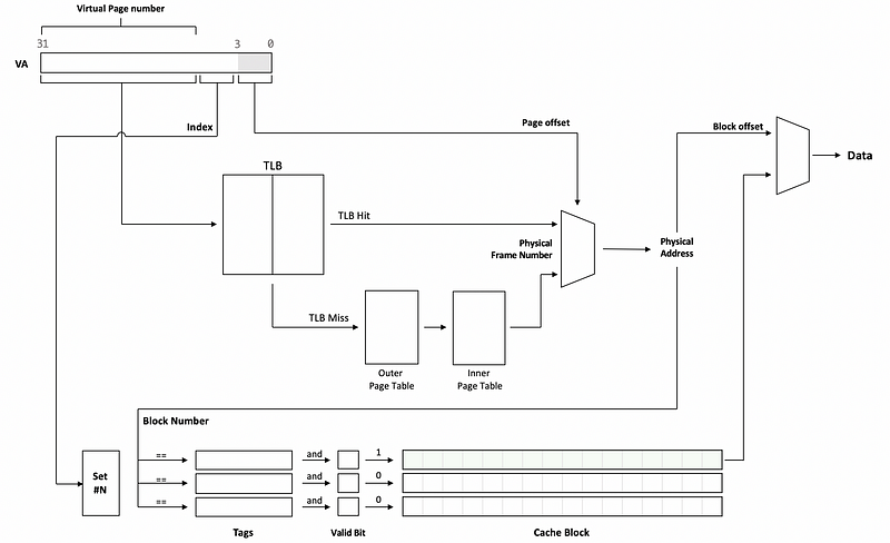
Hit time is also affected by having to access the TLB before we access the cache. This is because we always have to do the virtual to memory translation before we can have an access to the cache. You can refer to the following diagram to see how it works,
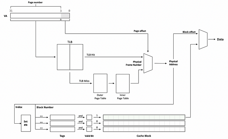
By this diagram, we can find out that if the TLB takes 1 cycle and the cache takes 1 cycle, we will need 2 cycles from when the processor gives us the virtual address (VA) until we actually get the data.
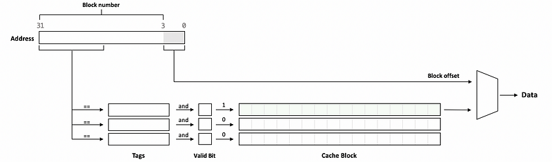
(3) The Definition of Physical Cache
As we have discussed, a cache that can only be accessed using the physical address is called a physical cache (aka. physically accessed cache, physical-indexed physically-tagged cache, PIPT cache). The overall hit latency of a PIPT cache is the TLB hit latency plus the cache hit latency,

In the diagram above, we can find out that both the set and the tags are compared against the bits from the physical memory, then this is why it is called a physical-indexed physical-tagged cache.
(4) The Definition of Virtually Accessed Cache
We can improve the overall hit latency by a virtually accessed (aka. VIVT or virtually-indexed virtually-tagged) cache. In that case, the virtual address is what we use to access the cache and get the data.
If we have a cache miss, then we would use the virtual address to index the TLB for telling us what the physical address is, so that we can bring the data back to the cache when we get it from the physical memory.
But for a cache hit, we don’t need to go to the TLB and do virtual to physical translation. The advantage of this virtually accessed cache is that the overall hit time will only be the cache hit time without the TLB latency,

It seems that the virtually accessed cache can surpass the PIPT cache in every aspect. First of all, the latency of the virtually accessed cache is lower because it doesn’t need to wait for the TLB access. Also, the energy will be reduced because it takes fewer operations.
(5) Problems For Virtually Accessed Cache (VIVT Cache)
So far, the virtually accessed cache seems good for us. But there are some problems.
Firstly, the page permission information will be stored in the TLB and that means if we don’t access the TLB, we will not know whether or not we have the permission of accessing a page. So it will be a must for us to access the TLB before we access the cache.
Secondly, a more serious problem is that different applications have different virtual memory addresses for the same data. This means that every time we conduct a context switch between the processes, the content in the cache can not be used anymore. Thus, we have to do a cache flush for every context switch. Although the cache flush can be quick, it will cause more cache misses and this adds to the overall cost.
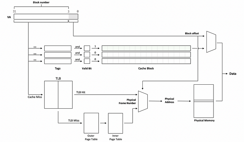
That’s why we design a virtually-indexed physically-tagged (VIPT) cache.
(6) Aliasing For Virtually Accessed Cache
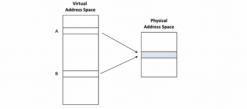
There is another serious problem for the VIVP called aliasing. Let’s see an example about aliasing. Suppose we have two addresses,
A: 0x 1234 5000
B: 0x ABCD E000
and we also have a 64 KB directed-mapped cache with 16-byte block size, and this cache is virtually accessed. Because the block size is 16 B, then we have a 4-bit offset. Also, because we have 2¹² entries in the cache (i.e. 64KB/16B = 2¹²), we have 12 bits for the index. The rest of the virtual address will then be the tags. So,
Addr               Tags        Index     Offset
---------------    --------    ------    -------
A: 0x 1234 5000    0x 1234     0x500     0x0
B: 0x ABCD E000    0x ABCD     0xE00     0x0
Let’s suppose that we have a write-back cache (means that the cache will not write to the memory immediately) and suppose that both the address A and B will be mapped to the same physical address. This can be legal for most operating systems if we use something like,
mmap(A, 4096, fd, 0);
mmap(B, 4096, fd, 0);
Assume that both A and B are not in the cache, then if we execute the following program,
WR A, 16
RD B
Because A is not in the cache, we will get a cache miss. Then we will translate A and grab its value from the memory and change the value in the cache from the origin (let’s say, 4) to 16.
Because B is also not in the cache, we will then translate B and then grab its value. However, since we haven’t written A to the memory, what we read from the memory is the original value 4 instead of the value 16.

The reason for this problem is that the caches are tagged by the virtual addresses and they can be different even for the same physical address. So VIVT caches need additional support for this problem. Any time we write to the virtual location, we have to do a check in case of an alias in the cache. However, this can be quite expensive to do, and it kind of defeats the purpose of virtually accessed caches.
(7) Methods for Reducing Hit Time #2: Virtually-Indexed Physically-Tagged (VIPT) Caches
So the main problem for the PIPT is that we must wait for the TLB hit, and the main problem for the VIVT is that we do not want to keep the cache for all the different applications, so there won’t be any cache flushes.
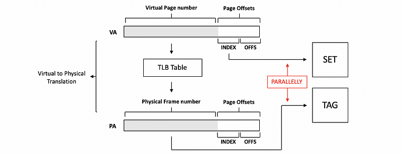
The VIPT is actually a combination of the advantages of the PIPT and the VIPT. We use the index bits from the virtual address to find the set we want in the cache, and then we read the valid bits and the tags from it. Meanwhile, we also use the page number to access the TLB and then get the frame number and translate the physical address. Now because we have the physical address, we perform the tag check using the physical address.
Note that the cache array and the TLB access can proceed parallelly, and because the TLB is fast enough because it is very small, the hit time will be equal to the cache hit time.

And because TLB hit latency < Cache hit latency, we have,

Also, it turns out that we don’t need to flush when we have a context switch. This is because the caches are checked by the physical address, not the virtual one. So even though the virtual address in another process may map to the same set, its page number may not match the tags.
(8) VIPT Aliasing
The VIPT will not have an aliasing problem because the virtual pages that will have different page numbers that map to the same physical frame number can have the same page offsets. If the index is only determined by the page offsets, then the index will not change during the virtual to physical translation.
So if all the index bits come from the page offset, we will not have any aliasing problems. To implement this, the caches have to be small.
For example, if we have a 4KB page, we will have a 12-bit page offset. If the cache has a 32 B block, then it has a 5-bit block offset. If now we want the index also fit in the page offset, it can only have 7 bits and this means that we can have only up to 128 sets in the cache. You can see that because we want to avoid the aliasing problem in the VIPT cache, we have to limit the size of our cache.
(9) VIPT Cache Size
Now, we have discussed the maximum index bits we can have to avoid an aliasing problem, then let’s discuss the maximum size of a VIPT cache. Let’s suppose that we have a 4-way set-associative cache with 16 bytes for each block. Assume that the page size is 8KB. Calculate the maximum VIPT cache size if we want to avoid aliasing.
Because we have a page size of 8KB, then the page offset must be 13 bits (i.e. log2(8*1024) = 13). Because we have a block of 16B, the block offset should be 4 bits (i.e. log2(16) = 4). The all the rest of the bits in the page offsets can then be used as the index, so we have 9 bits for the index and thus we can create 512 sets (i.e. 2⁹ = 512). Note that we because have a 4-way cache, which means that for each of the sets, we can have 4 blocks. So the overall size of the cache will be 32 KB (i.e. 512*16*4 B = 32 KB).
In a more general case, we can discover that the maximum number of sets we can create times the block will always equal the page size. This means that we can simplify our results. Regardless of the block size, the maximum cache size we can have will be the page size times the # of blocks in each set (i.e. the associativity of the cache). This is to say that,

(10) Real VIPT Caches
Now, let’s look at the sizes of some actual VIPT caches.
For Pentium 4 processor, it has a 4-way set-associative cache with a page size of 4 KB. So the L1 cache is designed to be 16 KB.
For a more recent Core 2, Nehalem, Sandy Bridge, or Haswell processors, they have an 8-way set-associative cache with a page size of 4 KB. So the L1 caches for these processors are designed to be 32 KB.
The upcoming Skylake designed processor from Intel has a 16-way set-associative cache with a page size of 4 KB. So its L1 cache is designed to be 64 KB.
(11) Relationship between Associativity and Hit Time
If we have a high associativity cache, we tend to have fewer conflicts, which leads to,
- a reduction of the overall miss rate: this will benefit the performance
- a larger VIPT cache size: this is explained above and it will also benefit the performance and leads to a lower miss rate
Also, because we have to search in the set for the cache hit, it will also lead to a higher execution time. This is slow and bad for the performance! However, because the simple direct-mapped cache has only one place to check for a single block, the execution time will be lower, but the direct-mapped cache sacrifices the miss rate because of the conflicts.
For reducing the execution time of a high associativity cache, we have to make some cheating on the associativity.
(12) Cheating #1: Way Prediction
One way of cheating on associativity is called the way prediction. The basic idea for the way prediction is that we can guess which line in the set is the most likely to hit and just check that one.
If we are right, then the hit time will be reduced to the same as a direct-mapped cache.
If we are wrong, then we will get no hits there in the line we guess. Then we will do a normal set-associative check on the other lines, which will have a high hit time.
So basically, for a way prediction method, we will first guess the hit line in the set, so it will be more like a direct-mapped cache. And if we make a wrong guess, we will then do what the normal set-associative caches do.
(13) Way Prediction Performance
Now, let’s see an example of how does the way prediction improves performance. Suppose we have the following three caches.
The first one is a 32-KB 8-way set-associative cache with,
- a hit rate of 90%
- a hit latency of 2
- a miss penalty of 20
The second one is a 4KB direct-mapped cache with,
- a hit rate of 70% (because it has a higher miss rate)
- a hit latency of 1 (direct-mapped can be faster)
- a miss penalty of 20
The third one is a 32-KB 8-way set-associative cache with,
- way prediction
- a hit rate of 90%
- a hit latency of 1 (when guessing right) or 2 (when guessing wrong)
- a miss penalty of 20
Let’s now calculate the AMAT for these three caches.
The first one can be calculated by 2 + (1 — 90%)*20 = 4. The second one can be calculated by 1 + (1 — 70%)*20 = 7. Compare these two results, we can find out that even though the direct-mapped cache has a smaller hit time, it can pay higher AMAT because of the reduction of the hit rate.
For the third one, firstly, we will first treat this cache as a direct-mapped cache so that we can have a 70% hit rate with 1 cycle latency each. For those who are missed in the direct-mapped cache, we will then use a normal set-associative cache. In this turn, all the rest 30% pay a 2-cycle latency some with them, 10% pays an extra 20-cycle latency because of the cache miss. Thus, the overall AMAT, in this case, would be,
AMAT = 70%*1 + 30%*2 + 10%*20 = 3.3
We can see that the performance improves compared with the set-associative cache without way prediction.
(14) Relationship between Replacement Policy and Hit Time
Recall that the replacement policy is the policy for deciding which line to kick out in a set.
A simple replacement policy (e.g. random policy) has nothing to update on a cache hit. When we have a cache miss, we start to implement our policy by randomly selecting a block in the set to kick out. This policy is good for the hit time because we don’t have to do extra checks. However, we pay a higher miss rate because we often kick out blocks that we will frequently use.
An LRU policy can result in a lower miss rate, but it has to updates lots of counters on every cache hit. So there’s a lot of activities on every cache hit that results from needing the state that will we use later. As a result, we will have to spend lots of power and we will also have slower hits.
So generally, what we want is to have a replacement policy that has a miss rate very close to LRU, but we want to do less activity on cache hits.
(15) Cheating #2: Not Most Recently Used (NMRU) Policy
The NMRU policy is an approximation of the LRU policy but it will have a better performance. The NMRU is implemented by recording the most recently used (MRU) line by a counter and randomly kicks out one of the NMRU lines.
If we have a 4-way set-associative cache, there will be 4 blocks in a set. For the LRU policy, we have to have 4 2-bit LRU counters to trace the LRU. However, we only need a single 2-bit counter if we implement the NMRU policy because we only need to record the MRU block. Generally, the NMRU keeps N times less than the LRU counters.
Although this NMRU policy does have a hit rate that is slightly lower than the LRU, the hit time can always be reduced significantly compared with the cost of the hit rate. NMRU is not perfect because it doesn’t track the rest of the blocks except for the MRU and it will conduct a random kick-out.
What we want is actually a policy that is still simpler than the LRU but keeps more track of what’s less recently than the MRU.
(16) Cheating #3: Pseudo LRU (PLRU) Policy
The PLRU is a policy that tries to approximate LRU in some way but it doesn’t exactly match the LRU. Instead of keeping the sequence of the usage frequency, the PLRU adds a bit for each block in the set to show that if it is recently used.
In the beginning, all these extra bits will be set to 0. When a block is recently used, this bit of it will be set to 1. After several times, we can find out that some of the blocks will have their bits set to 1 (means that they are recently used) and the other will have their bits remain 0. When now have to kick a block out, we only randomly choose from the lines that have their bit remains 0.
There is a situation when all the bits of the lines are set to 1. At this moment, we can not replace any of the lines in this set. So when we set the last 0 bit to 1, we will zero out the remaining bits. When we have only 1 bit set to 1 in a set, it is more like an NMRU policy. However, if we have more bits set to 1, this policy will be better than the NMRU policy because we know more than one MRUs.
Thus, this policy behaves somewhere in between the LRU policy and the NMRU policy.
3. Improving Cache Performance with Miss Rate
(1) The Causes of the Misses: 3Cs
Now, we will focus on how to reduce the miss rate. Generally, there are 3 reasons for causing a cache miss,
- Compulsory Miss: when a block is accessed for the first time, and this will happen even for an infinite cache
- Capacity Miss: blocks evicted when the cache is full. This is because we have a limited cache size.
- Conflict Miss: blocks are evicted due to associativity. This is because we have limited associativity.
(2) Methods for Reducing Miss Rate #1: Larger Cache Blocks
The first technique to reducing the miss rate is using larger cache blocks. This can reduce the miss rate because more words will are brought in when we have a miss, so the subsequential accesses on the words will not be misses. So this does reduce the miss rate only when the spatial locality is good. When the spatial locality is poor, the miss rate will increase because we bring in more words we don’t need.
So when we increase the block size, the miss rate will first reduce because it benefits from the spatial locality. But as we exhaust the amount of spatial locality, the miss rate will increase.

(3) Methods for Reducing Miss Rate #2: Prefetching
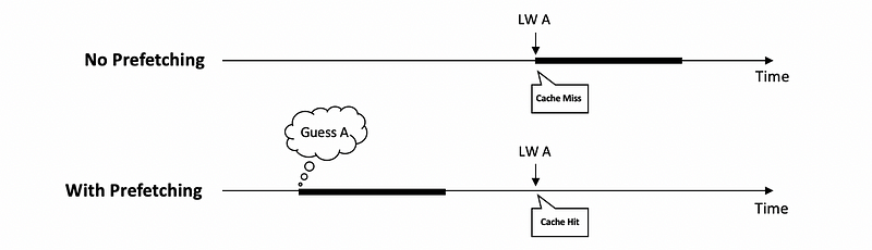
Another idea that uses a similar idea of the way prediction is called prefetching. The idea of prefetching is that we guess which block will be accessed soon in the future before they are actually accessed, and then bring those blocks into the cache before they are actually accessed. If our guess is right, when we request something from the memory for the first time, instead of a cache miss, we will have a cache hit. So there will be no need to wait for memory latency.
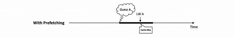
However, if our guess is wrong, we will then have cache pollution because we are bringing stuff that is useless into the cache. Another problem is that we not only don’t eliminate the cache miss, we may also kick out something that can be useful in the cache.
(4) Prefetching Instructions Implementation
The way to implement prefetching is to just add prefetching instructions, and let the compiler and the programmer figure out when to request prefetching. Let’s suppose we have the following program,
for (i=0; i<1000000; i++) {
    sum += a[i];
}
This program will access the elements in the array one at a time and then sum them up. So there will be a lot of spatial localities and we can improve the miss rate by prefetching. With prefetching instructions, the program will be something like this,
for (i=0; i<1000000; i++) {
    prefetch a[i+pdist];
    sum += a[i];
}
Where pdist here is a constant and it should be at least 1. Now our question is how to choose the value of this pdist?
- If
pdistis too small (e.g. 1), we may still have to wait for it because the memory access can not be that fast. This is a problem when the prefetch is too late.
- If
pdistis too large, although we may have this element in the cache ahead of time, it might be kicked up before it is finally accessed. So we will still have a cache miss. This is a problem when the prefetch is too early.

You can find that the coding of the pdist in the program becomes tricky because we can not have it too large nor too small. What’s more, the pdist is also related to the performance of the processor and the memory, which can be verified in every execution.
(5) Hardware Prefetching
Because we have some difficulty coding into the program for the prefetch, we can use another method called hardware prefetching, where the program doesn’t change, and the hardware itself tries what will be accessed soon. There are many hardware prefetchers that work pretty well. For example,
- Stream buffer: sequential in nature, so it just trying to fetch several blocks in advance
- Stride prefetcher: monitors the access and see if the memory we are accessing has a fixed distance between each other. Then it will prefetch the memory with this times of this fixed distance.
- Correlating prefetcher: predicts the sequence of the accesses. In a table, it will record the sequence of the memory accesses and try to prefetch the following accesses based on this table.
(6) Methods for Reducing Miss Rate #3: Loop Interchange
A final type of optimization for reducing the miss rate is called the loop interchange. This is one of the compiler optimizations that can be done to transform the code into a code that has a better locality. Let’s see an example. Suppose we have the following code,
for (i=0; i<N; i++) {
    for (j=0; j<N; j++) {
        a[j][i] = 0;
    }
}
Then when we access the memory in this nested loop, we are going to access some way like the following diagram,
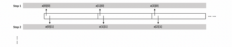
We can see that all the memory we accessed will have a distance from each other, and this is not good for us because we can not benefit from the spatial locality. So a good compiler will find this problem and compile the program above in another way,
for (j=0; j<N; j++) {
    for (i=0; i<N; i++) {
        a[j][i] = 0;
    }
}
We can see that the sequence of the loop will be switched and now we are nicely sequentially accessing the matrix which can make us benefit from the spatial locality. As a result, the hit rate will be dramatically improved.
However, this method is not always possible, because we can not do this for any loop.
4. Improving Cache Performance with Miss Penalty
(1) Methods for Reducing Miss Penalty #1: Overlap Misses
The first method we want to discuss for reducing the miss penalty is called the overlap misses. Let’s see an example.
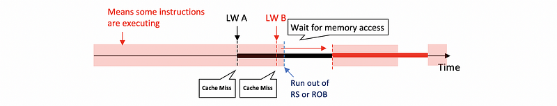
When we have a blocking cache (means that the cache will be blocked if we have a cache miss), in the beginning, we have some instructions executing. At some point, we perform a load instruction LW A, and A is not in the cache. So we have a cache miss and then we will start to access the memory for A. The program will be an out-of-order execution, so it will continue running.
However, because more and more instructions will rely on the result of A, then at some point we will run out of the RS or ROB. So the program can not continue to execute. Suppose there’s another load instruction LW B that occurs before the program stops, and B is also not in the cache. Instead of accessing the memory for B, this load instruction has to wait for the completion of LW A because we can only do 1 memory access at a time.
We can also have a non-blocking cache and it can support things like,
- hit under miss: meaning when we are having a cache miss, hit to the other blocks in the cache that are sent by the processor will be serviced and returned to the processor with data
- miss under miss: means that when we have a miss, we can send another miss to the memory. The property that the processor is exploiting here is called memory-level parallelism, and this means that we can have more than 1 access to the memory at a time.
Thus, the diagram for a non-blocking cache will be,
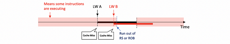
We can discover that with overlapped misses, we can have a better performance because we don’t have to pay the cost to wait for the memory access.
So what is most important is that we have to support the miss-under-miss execution or the memory-level parallelism in order to have a better performance.
(2) Miss-Under-Miss Support in Caches: Miss Status Handling Registers (MSHRs)
Before, the cache would simply block when it has a miss and not do anything until the miss comes. So it doesn’t need much support for that. However, with miss-under-miss, we have a miss but the cache will not be blocked. So other accesses keep coming to the cache.
If there are hits, we can handle them normally by just finding those blocks. If there are misses, we have to do more now. We ought to have miss status handling registers (MSHRs), and these are used to remember what we request from the memory.
(3) MSHR Implementation
The MSHRs keeps the information about the cache misses that we currently have in the process. So when we have a cache miss, we have to check the MSHR first to see if there’s any match. When we have a miss, we want to know whether it is a new miss or it is an existing miss waiting for the data back from the memory. So basically, we can have 2 situations,
- Miss: if there’s not a match in the MSHRs, we can know that it is a miss to a different block. In that case, we allocate a new MSHR where we remember which instruction in the processor to wake up when the data comes back
- Half-Miss: if there’s a match in the MSHRs, we can know that we try to find data from a block, and that block had at least one previous miss that was already sent to the memory but it didn’t come back yet. So because the request for this has already set to the memory, we should not do that again. Instead, we simply add that instruction to the corresponding MSHR. When the data comes back from the memory, we ought to wake up all the instructions that were added to this MSHR. After waking up the instructions, we release the MSHR that we have allocated for this data.
(4) MSHR Amount
So how many MSHRs we have to use? It turns out that there’s a huge benefit for us even if we only have 2 MSHRs so that we can handle two different block misses at the same time. It would be even better if we have 4 MSHRs. Moreover, even if we have 16 or 32 MSHRs, we can still benefit from the MSHRs.
(5) Methods for Reducing Miss Penalty #2: Cache Hierarchy
The method of cache hierarchy is also called the multi-level caches. We have already discussed the L1 cache, which is considered to be the first level for a cache hierarchy. When we have a cache miss in the L1 cache, we will just go to another cache.
(6) AMAT with Cache Hierarchy
So suppose we have an L2 cache, and when we have a cache miss in L1, we will then go to search in the L2 cache. So, the miss penalty for the L1 cache is not equal to the memory latency. Instead, it will equal to,

We can even have more levels of cache. Then the miss penalty for the rest of the level should be,

Note that if we have a cache miss in the last level cache (LLC), we have to go to the memory and find the data we need. So the miss penalty for the last level cache would be,

(7) Multi-level Cache Performance
Suppose the memory latency is 100 cycles and for the following 4 types of caches, let’s calculate the AMAT for each of them.
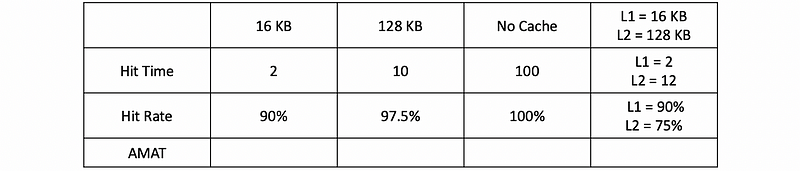
After calculation, the final results would be,
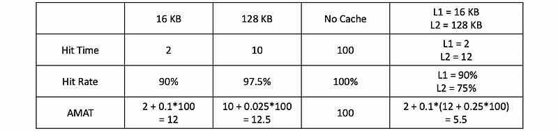
We can find out that the cache hierarchies work better than individual caches and why we have them. It is not enough to have only a large cache or a small cache. In that case, you can combine the caches to have a better performance.
(8) Global Hit Rate Vs. Local Hit rate
We can find out that the hit rate of L2 (i.e. 75%) in the cache hierarchy is lower than the result if we only have a 128 kB cache (i.e. 97.5%). This is because, in cache hierarchy, the L2 is only accessed by the data that is missed in L1, and this makes it even harder to predict.
A local hit rate is a hit rate that the cache actually observes. Because all the accesses to the L2, L3, and etc. caches (except for L1) do not benefit from localities, the local hit rate is lower compared with the global hit rate (means when such a cache is used alone).
- Global Hit Rate

- Global Miss Rate

- Local Hit Rate

- Local Miss Rate

(9) Misses Per Thousand Instructions (MPKI)
Another popular metric of how often the cache hits that tries to capture the behavior of caches that are not the L1 cache is misses per thousand instructions (MPKI). It is very similar to the global miss rate except that it doesn’t normalize the misses with the number of memory accesses. It normalizes with a number of instructions.
(10) Inclusion Property for Cache Hierarchy
Now, let’s discuss the last topic of the cache hierarchy, the inclusion property. When we have a block that exists in the L1 cache, there can be three situations in the L2 cache,
- Inclusion: means that this block is also in the L2 cache
- Exclusion: means that this block is not in the L2 cache
- Random: means that this block may or may not be in the L2 cache
Except for the case that we explicitly point out it is an inclusion or an exclusion, most cache hierarchy will result in a random state. So the inclusion and the exclusion don’t necessarily hold for this case because things that accessed in the L1 cache will not access the L2 cache.
To force an inclusion, we need to add a bit for inclusion.