High-Performance Computer Architecture 28 | Introduction to Fault Tolerance, Memory and Storage …
High-Performance Computer Architecture 28 | Introduction to Fault Tolerance, Memory and Storage Fault Tolerance, RAID
1. Introduction to Fault Tolerance
(1) The Definition of the Dependability
Dependability means the quality of a delivered service that justifies relying on the system to provide the service. So a dependable system is the one that provides the service in a way that makes us expect it to do provide the correct service.
(2) Two Kinds of Servies
The service we have talked about actually has two definitions.
- Specified service: what the behavior of the system should look like (the expected behavior)
- Delivered service: the actual behavior that the system provides
We can also conclude that dependability is about could we say that the specified service matches the delivered service.
(3) System Components
The system components (aka. modules) are some largish components in our computer like the processor, the memory, and so on. For each of these modules, we can specify some behavior that it should ideally get. So when we talk about things that make things not be so dependable, we are really talking about modules deviating from the specified behavior and thus, the delivered service no longer matches the specified services.
(4) The Definition of Fault
The faults (also called the latent error) happen when the modules deviate from the specified behaviors. The most common fault is a programming mistake. For example, suppose we have an add function that works really well except for the case 3+5=7. This fault may not occur at the beginning, but it is just a matter of time.
(5) The Definition of Error
The error (also called activated fault, effective error) happens when the actual behavior within the system differs from the specified behavior. For example, we call the add function that we have talked about and add 3 to 5. Result 7 is put in some other variable.
(6) The Definition of Failure
The failure occurs when the system deviated from the specified behavior. For example, when we want to schedule a meeting time at 8 but we finally scheduled the time to 7 because of the error in the function we have talked about.
(7) Difference between Fault, Error, and Failure
We should keep in mind that all not all faults will become errors, and only those activated faults will become errors. Similarly, we can have an error sometimes, but not all the errors will become failures.
(8) The Definition of Reliability
There are some other properties in fault tolerance, and one of them is called reliability, which is something we can measure. In order to measure the reliability, we consider the system in one of the following two states,
- Service accomplishment state (the normal state)
- Service interruption (the service is not providing)
The reliability can be defined by measuring the continuous service accomplishment states, and a typical measure is called mean time to failure (or MTTF). This is basically how long do we have service accomplishment before we get into the next service interruption.
(9) The Definition of Availability
The availability measures service accomplishment as a fraction of the overall time. So reliability measures how long do we get from the service accomplishment until the next failure, the availability measures what percentage of time we are in the service accomplishment state.
For the availability, we have to know the main time to repair (or MTTR). This is once the service has interrupted, how long does it last until it goes back to the service accomplishment state. So the availability can be calculated by the MTTF divided by the sum of MTTF plus MTTR,

(10) Different Types of Faults
We can classify the faults by different causes, these contain
- Hardware (HW) faults: hardware fails to perform as designed
- Design faults: like the software bugs, or the hardware design mistakes (e.g. FDIV bugs)
- Operation faults: operator or the user’s mistakes. For example, an operator mistakenly shut down the service
- Environmental faults: like the fire and the power failure
Or we can also classify the faults by duration, which means how long do we have the fault condition,
- Permanent faults: once we have it, it doesn’t get corrected
- Intermittent faults: last for a while but recurring (e.g. if we overclock the system)
- Transient faults: last for a while and then go away
(11) How to Improve Reliability and Availability?
There are actually several things we can do to improve the reliability and the availability of the system. We can try to,
- Avoid faults as much as we can: preventing faults from occurring
- Tolerance of some faults: prevent faults from being failures (e.g. Error-correcting code)
- Speed up repair: which only affects availability.
(12) Fault Tolerance Techniques
In order to improve the reliability and the availability, we can use some fault tolerance techniques like,
- Checkpoints: the checkpointing saves the state periodically, then if we detect the errors, we will stop the system and restore the state. This technique works well for many transient and intermittent faults. However, if the checkpoint takes too long to recover, this will be treated as a service interruption.
- 2-way Redundancy: (also called dual-module redundancy, or DMR) we can also use the technique called the 2-way redundancy where two modules do the exact same work. After each service, we will compare the results of them and we will roll back if the results are different. This is an error detection technique and it should be associated with the recovery techniques like checkpointing.
- 3-way Redundancy: (also called triple-module redundancy, or TMR) but with a 3-way redundancy, we can both detect and recover some faults. In this case, three modules are going to do the same work and they will vote for what the correct result should be. If one module is malfunctioning, then the other two will still produce the same result and that result will be elected as the correct result. Although the implementation of this design is expensive, it can actually tolerant any fault in 1 module.
- N-way Redundancy: a more general redundancy approach is called an N-way redundancy. If N = 5, there will be 5 votes. If we have one wrong result in a vote, we can tolerant this fault and we can continue the normal operation. If we have 2 wrong results in a vote, although we will have no failure, we will abort the current mission. This is because that we are confirmed that 2 out of 5 modules must have some faults and if we continue, we may have one more module with faults, and then we can not safely land the space shuttle.
2. Memory and Storage Fault Tolerance
(1) Overkilling Problem for Memory and Storage
Now, let’s see some fault tolerance techniques for memory and storage. We could use DMR or TMR for memory and storage. But these techniques are considered to overkill for these devices because DMR and TMR are typically used for the hardware that does the computation. Thus, we have to figure out some better techniques for this problem.
(2) The Definition of Codes
The error detection technique developed only for the memory and the storage is called the error-correction code. The idea is that we can store some extra bits (we call it code) that allow us to perform fault detection and correction depending on the code.
(3) The Definition of Parity Bit
The parity bit is the simplest code that has only 1 bit, and it can be calculated by simply XOR all the data bits. When we do have parity and the fault flips only 1 bit, then the parity code will no longer match the data.
(4) The Definition of Error-Correction Code (ECC)
The error-correction codes are the more complicated ones with more than 1 bit. A typical ECC is called the single error correction, double error detection (aka. SECDED) code. This code will correct it if there’s only a 1-bit flip, and this code will also figure out that there is a fault if we have a 2-bit flip.
(5) Reed-Solomon Error-Correction Code for Hardware
This code is even fancier and it is used mainly by the hardware (e.g. disks). This code can detect and correct multiple bit errors and they are especially powerful when we have a streak of flipped bits, which happens when the magnetic head isolate the platter for a little bit while it is spinning and misses some of the bits. We are not going to take about this in detail.
3. RAID
(1) The Definition of Redundant Array of Independent Disks (RAID)
RAID is another technique family that we commonly used for error correction, which stands for redundant array of independent disks. The fact of the RAID is that we have several disks that play the role of only one disk in different ways. They can either pretend to be a larger disk, or they can pretend to be a more reliable disk, or they can pretend to be a disk that is both larger and more reliable than we have only one disk.
Each of the disks in a RAID model will still detect the error using codes so that we can know which and whether a disk has an error in the RAID scheme. So what we want from RAID is a better performance and we want normal read-write accomplishment even when there are bad sectors on disks or an entire disk fails.
Not all the goals we have mentioned will be implemented by only one RAID, so we have several RAIDs and we name them as RAID 0, RAID 1, RAID 2, etc.
(2) RAID 0: Striping
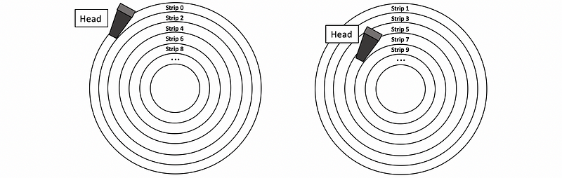
The RAID 0 uses a technique called striping to improve performance. If we have one disk, it will turn out to have track 0, track 1, track 2, … on that disk. The magnetic head will read through the whole track and then the data can be retrieved from the track. However, this can be inefficient because we can not read from a track and moving the head to another at the same time.

The RAID 0 deals with this problem by using a technique called striping. What it does is to write tracks on two different disks and treat them as a whole, larger disk. Now, these “track”s on different disks are called strips instead of the track to avoid confusion with the track on the physical disk. On average, the performance (throughput) will be twice because we can read from one disk and move the head of another disk, and we can also read simultaneously from both of the disks at the same time. When the first read finishes, we can immediately read from the second disk without any latency for moving the heads.
However, the reliability of the RAID 0 is getting worse. Let’s assume f is the failure rate for a single disk, which is defined by the number of failures per disk per second. Obviously, this number will be extremely small. Usually, we can assume that the failure rate is constant over time. So the MTTF of a single disk can be calculated by,

When we have N disks in RAID 0, the failure rate for each disk will be f and in general, we will have a failure rate of Nf, so the MTTF, in this case, would be,

As a result, we can find out that the MTTF with N disks in RAID 0 is N times smaller than the MTTF with a single disk. When N is getting larger and larger, we will have a really small MTTF limit to 0, and the machine is not reliable anymore.
(3) RAID 1: Mirroring
The next RAID technique is RAID 1 and it uses a technique called mirroring to improve reliability. We will have a copy of the data on another disk, so this means that each disk will have the same write. So each disk does exactly the same writing that they will be doing.
However, when we read from the disk, we will read from only one disk because both of the two disks contain the same data. Now, if there is a bad sector on one disk, we can just read the same data from the other disk. Or if we have an entire disk fail, we are also left with a disk that still has all the data we can read. We don't compare these to disks to detect errors because the ECC is already assigned to each disk. So that we can just read from the correct disk.
Now let’s talk about the reliability problem related to RAID 1. Suppose the RAID 1 has 2 disks and the failure rate is f. Then the MTTF for the entire 2 disks (one for the copy) as we have discussed with the same content should be,

However, after the first disk fails, we are going to have an MTTF of a single disk, which is exactly,

Therefore, the overall MTTF of our system should be,

In the example above, we have assumed that no disk is replaced after we detect a fault, which is actually not the case in reality. Well, in reality, we will definitely replace the fault disk immediately and then there will not be a problem.
So how can we calculate the MTTF when considering the fact that all the fault disks are replaced properly? The answer is that we have to consider the repairing time (MTTR). Let’s reconsider the 2-disk RAID 1 system. In the beginning, the MTTF of the entire system would be,

After the first disk fails, we have to replace it with a new disk so that it will be working later. During the repairing time, we will only have one disk, but because the MTTR (for days) is relatively small compared with the MTTF (for years), we can ignore the process of a single disk and just consider it as two disks working all the time.
Then the overall MTTF will be MTTf_2 times the times of repairings until we can not finish one in the MTTF time. So in general, the result will be,

(4) RAID 2&3: Not going to talk about
We are not going to talk about RAID 2 and RAID 3 because they are rarely used today.
(5) RAID 4: Block Interleaved Parity
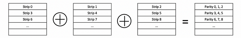
The RAID 4 uses a technique called block interleaved parity (aka. BIP). The content of this technique is similar to RAID 0 which separates different tracks as strips on different disks. The only thing that is different is that it adds an additional disk which is used for keeping the XOR results of strips as parities.
So when we write to the disk, we are actually writing to both the stripe and the parity. When we read from the disk, we are actually reading from only the corresponding disk.
Now, let’s see the overall performance of RAID 4. The throughput of reading from RAID 4 is N-1 times larger than the throughput of a single disk because we can read from N-1 disks simultaneously. However, the writing throughput is much worse than that because we have to write to both the corresponding disk and the parity disk. As a result, the writing throughput will be halved. This is also the reason why we need RAID 5.
In fact, the RAID 4 write is not as simple as that, we also have to consider how we can update the parities. Let’s see if we have a new stripe value for a 5-disk RAID 4 system (including 1 as the parity disk), one idea for generating the parity is that we simply read from the other 3 disks and then conduct XOR calculations. However, in this process, we have to conduct 3 reads (from the other 3 disks) and 2 writes (write to both the corresponding data disk and the parity disk). You can see that this is such a bad idea.
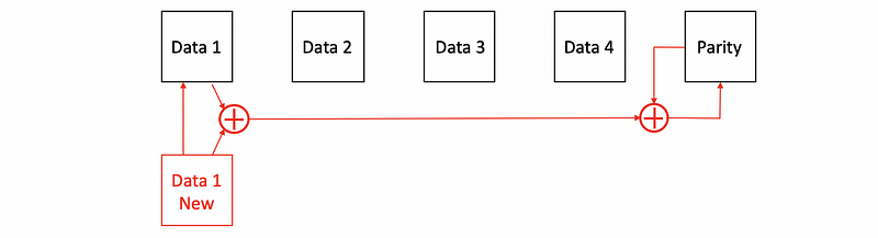
What can we do to reduce the reads and writes for RAID 4 is that we will not read from the other disks. What we can do is that we first read from the old data we would like to write, then we conduct an XOR between the old data and the new data. This XOR helps us finding the flipped bits between these two data disks. Then we will conduct an XOR between the flipped bits and the parity. Before we do so, we have to read from the parity first. After we calculate the result, we will write it back to the parity.
The reliability of the RAID 4. Again, all the disks are okay at the beginning until the first fault.

Then the fault appears in some disk and then we are willing to replace the disk with that fault. Similar to the last example, we can have an overall MTTF of

(6) RAID 5: Distributed Block Interleaved Parity
The RAID 5 is similar to RAID 4, but the parties are distributed among all the disks.
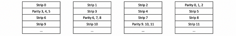
Because we can now read data from all of these N disks, we can confirm that the reading throughput will be N times the throughput of a single disk. A single write is also going to result in 4 accesses (2 reads and 2 writes) per write. But because the write is also distributed among 4 disks, we can have N/4 times the throughput of a single disk.
The reliability of RAID 5 is exactly the same as RAID 4.
(7) RAID 6
There is actually a RAID 6 in addition to the RAID 5. And what is different is that the RAID 6 adds another parity for each group of strips and this newly added check block is used for recovering when we have 2 disks failed. When there is only 1 disk failed, we can use the original parity for recovery. And when there are 2 disks failed, we can solve some equations of the original parity and the check block for recovery.
RAID 6 has twice the overall overheads to RAID 5 and we have to pay this for improving the reliability. There are more overheads per write because we have to write to both the parities and the check blocks. So now there are 6 accesses per write including 3 reads and 3 writes.
The RAID 6 is only used for the situation that we have a disk fails, and then we expect another fails before we replace the first disk. However, if all the faults are independent, it is unlikely that we have another disk fails when we are replacing the fault disk. So the RAID 6 is considered to be an overkill.
In fact, there are some cases when the failures are dependent. For example, we mistakenly replaced a correct disk and the fault disk still remains. In this situation, we will probability have 2 fault disks and if we have a RAID 6 system, we are able to recover from it.