Intro to Machine Learning 2 | Linear Model Regularization and Various Types of Gradient Descents

Intro to Machine Learning 2 | Linear Model Regularization and Various Types of Gradient Descents

Acknowledge: Thanks to Terence Parr, the professor of the University of San Francisco who made these cool visualizations. You can find these fancy pictures on his blog. Thanks to Lili Jiang and the gradient visualization tool she built, we can have these cool pictures about some different gradients methods.

1. The Definition of Regularization

Regularization is a form of statistical tool that constrains, regularizes, or shrinks the coefficient estimates towards zero.

2. Benefits of Regularization for Linear Models

Commonly, regularization has three main benefits,

• Prevent overfitting
• Increase generality
• Reduce model variance of estimates

3. Downsides of Regularization for Linear Models

Increase bias (the amount that a model’s prediction differs from the target value). This is not serious but the consequence is that we no longer know the effect of x_i on target y via β_i. So the method of regularization seems like we trade bias to get a lower variance.

Here is a picture showing the relationship between bias and variance.

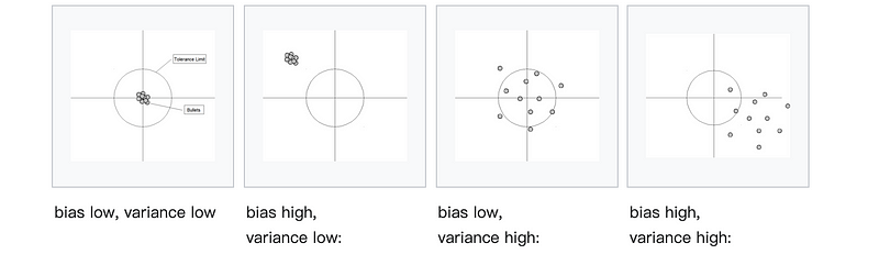
And here is another figure that shows why we can not achieve good bias and good variance at the same time.

The expected prediction error decomposition should be as follows,

4. Regularization Methodology

The idea behind regularization is to restrict the size of coefficients with hard constraint or soft constraint using the penalty term.

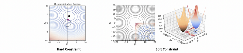
• Hard constraint: this is a conceptual statistical method and we have to construct a safe zone (which is the constraint of the coefficient) for finding the loss minimum. The minimum loss is inside the safe zone or on the zone border.

• Soft constraint: soft constraint is to add a penalty in the loss function by Lagrange multipliers so there’s no hard cutoff.

5. Why do we need to apply normalization/standardization for regularization?

Note that the concept of normalization or standardization here means the same thing, which is to scale the raw data by centered around the zero mean with a unit standard deviation (i.e. stdev = 1). The concept of normalization in sci-kit learn is quite different and what we are referring to is the StandardScaler.

Basically, we must apply normalization/standardization before regularization for two reasons,

• It leads to faster training: This is because we can go downhill in a rapid way. Loss contours for normalized variables are more spherical, which leads to faster convergence. See this paper.

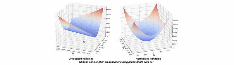
• It is required by regularization: the process of standardization is needed for generalization purposes, or the regularization shrinks coefficients disproportionately

6. Ridge Regression

Ridge regression adds an L2 regularization penalty to the loss function, which equals the square of the magnitude of coefficients.

On mathematics, the OLS estimate is,

And the Ridge estimate is,

7. L1 Lasso Regression

Lasso regression adds an L1 regularization penalty to the loss function, which equals the absolute value of the magnitude of coefficients.

Lasso is called so because the acronym LASSO stands for Least Absolute Shrinkage and Selection Operator.

8. Differences Between L1 and L2 Regularization

Both L1 and L2 increase model bias.

L1 encourages parameters shrinking to zeros, so it is more useful for variable or feature selection as some parameters go to 0.

L2 is more balanced or shrinks evenly (i.e. it discourages any parameter bigger than the other parameters) and is more useful when we have collinear features. This is because L2 reduces the variance of estimate parameters which counteracts the effect of collinearity

9. Turning Parameter (aka. Penalty Parameter) Selection

The turning parameter λ controls the strength of the L1/L2 penalty term.

• When λ increases, we can achieve lower variance but we pay higher bias.
• When λ decreases, we can achieve lower bias but we pay higher variance.
• When λ is 0, we remove the penalty term and the regularization turns off.

Particularly, when we have L1 regularization,

• When λ increases, we have more parameters shrinking to 0.
• When λ decreases, we have fewer parameters shrinking to 0.
• When λ is infinite, all the parameters shrink to 0.

To select a good turning parameter λ, we have to find it by computing the minimum loss for different λ values, then pick λ that gets min loss on the validation set.

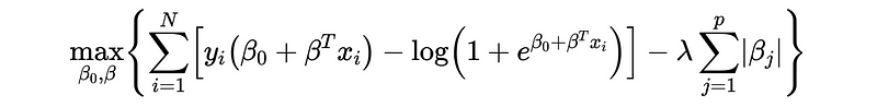
10. Regularized Logistic Regression

The L1 and L2 regularization for the logistic regression have exactly the same mechanism.

However, according to the ESLII book (page 125), we don’t want to shrink β_0 too small because it doesn't affect the variance as we expected. This means we must find β_0 different than the other parameters.

Commonly, we will directly assign β_0 as the mean value of y, assuming zero-centered data set.

11. Gradient Descent

• Slope (change in loss or β_i) in direction β_i: is the partial derivative

• The gradient is a p or p+1 dimensional vector of partial derivatives. For example, for a 2D gradient,

• The direction of the gradient is dependent on the sign of the slope, which points towards higher loss. So the gradient should therefore step by the negative of the gradient in order to find the minimum value.

where η is called the learning rate.

12. Learn Rate Selection

Learning rate selection is a trade-off between the rate of convergence and overshooting.

• When η is too large, we can go nowhere and β can even diverge
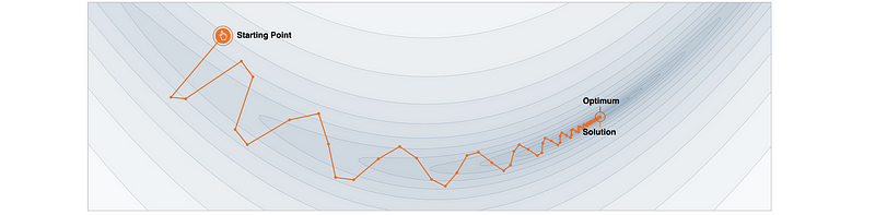
• When η is large, β oscillate across the valley
• When η is too small, β doesn’t make much progress towards min loss point and it may take too long to converge or stuck in the local

To select a good η, we have to find it by computing the minimum loss for different η values, then pick η that gets min loss on the validation set.

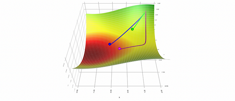
13. Different Types of Gradient Descent

• Vanilla Gradient Descent: the simplest version

Repeat:

Until:

Return:

• Gradient Descent with Momentum: record the historical steps and apply an impact of it on the current step. There are two benefits of applying a momentum gradient descent: (1) it moves faster than vanilla with the same learning rate (but the general consumed time is uncertain because it may take a longer distance); (2) it has a shot at escaping local minima because of the impacts of historical steps were added.

Repeat:

And then:

Until:

Return:

where the momentum hyperparameter γ is a new hyperparameter and it is usually set to 0.9 or a similar value.

• Adaptive Gradient (aka. AdaGrad): sometimes when we have a saddle plane, the momentum approach may not be our best method to choose. This is because it takes a detour towards the minima.

The AdaGrad method is quite simple, which basically allows us to scale the gradient (i.e. normalize the partial directive on each parameter) so that we can get a balanced value. This is done by dividing each partial directive of the parameters with its square root with history.

One problem of AdaGrad is that it is too slow because we scale the gradient to the standard magnitude. To deal with this problem, we have to choose either a larger learning rate η or we have to leverage more tricks to this approach.

Repeat:

And then:

Until:

Return:

• Root Mean Square Propagation (aka. RMSProp): As we have discussed, the problem of AdaGrad is that this is too slow, and it is even slower when we have many steps! This is because the square sum of historical steps only increases and never shrinks.

The idea of RMSProp is that the current step is more important than the historical steps, so we can shrink the sum of historical step squares in each step by adding a hyperparameter decay rate ρ in [0, 1) (e.g. ρ = 0.9). The historical sum of squares will be scaled smaller by ρ and the current square will be scaled larger by (1-ρ).

Repeat:

And then:

Until:

Return:

• Adaptive Moment Estimation (aka. Adam): The Adam approach takes the advantage of both the Momentum and the RMSProp, which means it is not only rapid but shrinks directly without detour.

Adam introduces two hyperparameters of the decay rate, β_1, and β_2. β_1 is used to decay the historical values for the sum of the gradient, while β_2 is used to decay the historical values for the sum of the squared gradient.

Repeat:

And:

And then:

Until:

Return:

14. Common Gradient Formulas

• OLS Linear Regression

• LASSO Regression (L1)

• Ridge Regression (L2)

• Logistic Regression

• L1 Logistic Regression: we have to compute β_0 and β in different ways, which can be a little bit tricky.

15. Other Frequently Asked Questions

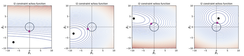
(1) Why L1 is more likely to shrink the parameter to 0 than L2?

In mathematics, the parameter in L1 regularization can quickly converge to 0 for a large λ. However, the parameter in L2 regularization struggles to converge to 0 for large λ.

(2) Is L1 always better than L2 or vice versa?

No. But if we currently don’t know anything else, we should choose L1 because it makes our model simple.

(3) Is it okay to get rid of L1 parameters that go to zero?

Yes, because they don’t contribute to the regression or classification.

(4) Why the loss function for regression is a bowl?

This is because of the definition of MSE, where the coefficients have squared values.

(5) Where to start gradient descent from a loss function?

It doesn’t matter, and we just start from some random point.

(6) Where to stop gradient descent?

We stop iteration when the loss is smaller than some threshold approximately equals 0 (i.e. flat)(we can not let it become exact zero because we may never reach that point with a given learning rate).

(7) How can we make sure that we find a global minimum?

By momentum or deep learning.

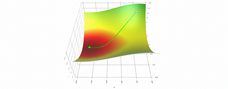
(8) Notice β accelerates and then slows down while iterating in gradient descent. Why?

When β is far from the minimum point, the absolute slope (gradient) is large, which means it can move a larger step along the curve in an iteration. When β is close to the minimum point, the absolute slope (gradient) gets smaller and the step becomes smaller.