Intro to Machine Learning 4 | Non-Parametric Models and Decision Tree
Intro to Machine Learning 4 | Non-Parametric Models and Decision Tree

- Parametric Models Vs. Non-Parametric Models
Parametric models have a finite number of parameters depending on the feature properties. For example, suppose we have N boolean features (i.e. X) and a boolean label (i.e. Y)
- Logistic Regression: N+1 parameters
- Navie Bayes Classifier: (2N + 1) * 2 parameters
- Neural Nets
Non-parametric models mean we have an unbounded number of parameters depending on the dataset. This means if the number of model parameters changes with different N records, it’s nonparametric.
- kNN
- Random Forest
- Gradient Boosting Machine
2. k-Nearest Neighbourhoods (kNN)
kNN is less often used in practice, but it’s knowing how they work and kNN can still be very effective,
- kNN Regressor: get k observations closest to unknown x using Euclidean distance then predict average y from those k’s
- kNN Classifier: get k observations closest to unknown x using Euclidean distance then predict the most common class from those k’s
The benefits of kNN are that,
- No Training Period: the kNN learns from the training set only when it makes predictions
- New data can be added seamlessly
- Easy to implement
The downsides of kNN are that,
- Does not work well with large sets: the cost of calculating distance can be very high
- Does not work well with high dimensions: it is more expensive to calculate the distance for high dimensions
- Need feature scaling: the kNN approach requires standardization and normalization
- Sensitive to noise: need extra work for removing outliers and missing values
3. kNN Vs. Decision Tree
One critical reason why we don’t use kNN in practice is the high cost of calculating the Euclidean distance.
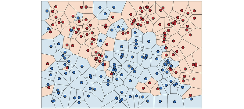
To make the boundaries easier, let’s avoid inefficiency and the distance metric requirement of kNN by partitioning feature space into rectangular hypervolumes and then predicting the most common y (or label) in a hypervolume. These partition rules can be encoded as a tree called a decision tree. With the help of the decision tree, we can deal with the following problems,
- Multiple Records Tolerance: just put similar records in the same leaf
- Deal with Inexact Feature Match
- Reduce the High Cost of Calculating Distance
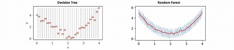
However, the decision tree still has a bunch of problems,
- Overfitting: if there are no other constraints, the decision tree tends to split the feature space by rectangular hyper volumes until each leaf has a single observation. We commonly deal with it by adding constraints, enhancing bagging (using bootstrapping for weakening a decision tree), or assembly randomness (also called ensemble learning, e.g. random forest).
4. The Structure of Decision Tree
- Growing Direction: Upside down
- Root Node: root node is the topmost node in a tree data structure
- Internal Node (aka. split): internal nodes have one or more child nodes, and they are used to test features (or test variables at split points)
- Leaf Node (aka. leaf): leaf node has no child nodes, and they are used to predict the region mean (for regressor) or predict the most common target category or mode (for classification)
- Layer: each stage of nodes is called a layer, for example in the following figure, we have 3 layers
- Depth: how many layers do we have in the tree

5. Different Splitting Methods
- Variance Reduction (Mean Square Error, MSE): for Decision Tree Regressor
MSE for the mean model is the same as variance, and this technique can be used to split the node.

- Entropy Reduction: for Decision Tree Classifier
Entropy is a way to measure the chaos within the system, and a higher entropy means a higher uncertainty of the class y in that sample. So we have to reduce the entropy if we want to purify the sample.

- Gini Impurity Reduction: for Decision Tree Classifier
Gini Impurity is another technique we can use to measure the class purity of a sample. It measures the uncertainty of the class y in that sample. Higher Gini Impurity means the sample is more uncertain, so we have to reduce the Gini Impurity if we want to purify the sample.

Note that Gini Impurity is similar to entropy but faster,

Let’s now see an example. Suppose we have a node sample of five values y = [1, 1, 1, 2, 0], and the predicted value of this node is 1.
The variance of this sample should be (if regressor),
variance = (0 + 0 + 0 + 1 + 1) / 5 = 0.4
The Gini Impurity should be (if classifier),
Gini Imputrity = 1 - (9/25 + 1/25 + 1/25) = 14/25 = 0.56
The Entropy should be (if classifier),
Entropy = -(log_2(3/5)*3/5 + log_2(1/5)*1/5 + log_2(1/5)*1/5)
= 1.37
6. Decision Tree in Python
The decision tree model can be applied for regressing or classifying. In sklearn, these are,
- Decision Tree Regressor
from sklearn.tree import DecisionTreeRegressor
- Decision Tree Classifier
from sklearn.tree import DecisionTreeClassifier
(1) Splitting Methods
For the regressor, the splitting method is defined by criterion and we can choose among,
criterion = [“squared_error”, “friedman_mse”, “absolute_error”, “poisson”]
And the default one is squared_error , which is the MSE we have discussed.
For the classifier, the splitting method is also defined by criterion and we can choose between,
criterion = [“gini”, “entropy”]
The default one is the Gini Impurity and we can change it to Entropy.
(2) Hyperparameters
As we have discussed, the decision model always overfits, and we have to develop some methods for increasing the generality.
max_depth: the depth of the tree. Decrease to avoid overfitting, and increase to increase accuracymin_samples_leaf: the minimum sample size per leaf. Increase to avoid overfitting, and decrease to increase accuracymax_features: the number of features to consider when looking for the best split. Decrease to avoid overfitting, and increase to increase accuracymin_samples_split: the minimum sample size we need for a split. Increase to avoid overfitting, and decrease to increase accuracy
(3) Plot the Decision Tree
import matplotlib.pyplot as plt
from sklearn.tree import DecisionTreeClassifier
from sklearn import tree
# Generate X and y
X_train = []
X = sorted([random.uniform(-3, 3) for i in range(50)])
for i in X:
    X_train.append([i])
y = []
# Partition rules
for value in X:
    if value < -1.3:
        y.append(0)
    elif (value >= -1.3 and value < -0.3):
        y.append(random.randint(0,1))
    elif (value >= -0.3 and value < 0.3):
        y.append(1)
    elif (value >= 0.3 and value < 1.3):
        y.append(random.randint(1,2))
    else:
        y.append(2)
clf = DecisionTreeClassifier(min_samples_leaf=10)
clf.fit(X_train, y)
fig, ax = plt.subplots(1,1,figsize=(8,8))
tree.plot_tree(clf, ax=ax)
plt.show()
The output would be (this result can be different because we generate our training set randomly),

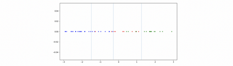
(4) Plot the Decision Boundary
colors = ["b", "r", "g"]
fig, ax = plt.subplots(1,1,figsize=(10,5))
for i, value in enumerate(X):
    ax.scatter(value, 0, c=colors[y[i]], alpha=0.5, lw=0)
for i in clf.tree_.threshold:
    if i != -2:
        ax.axvline(i, lw=0.4)
plt.tight_layout()
plt.show()
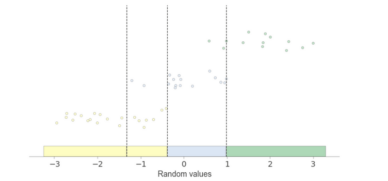
(5) Plot the Decision in a Better Way by dtreeviz
By using the dtreeviz Tool, we can draw some better graphs about decision trees. For example,
from dtreeviz.trees import *
viz = dtreeviz(clf,
               np.array(X_train), np.array(y),
               feature_names = "Random values",
               target_name='Partition Rule')
viz
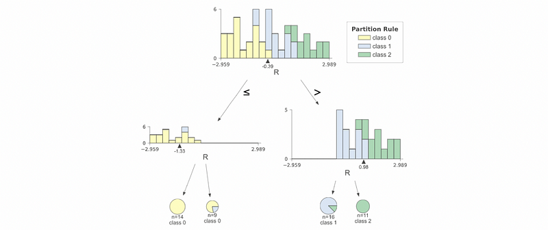
fig, ax = plt.subplots(1, 1, figsize=(10,5))
viz = ctreeviz_univar(clf,
                      np.array(X_train), np.array(y),
                      feature_names = "Random values",
                      target_name='Partition Rule',
                      show={'splits'},
                      ax=ax)
plt.show()