Intro to Machine Learning 8 | Data Processing Methods
Intro to Machine Learning 8 | Data Processing Methods

- Handling Missing Values
(1) Types of Missing Values
- Missing completely at random (MCAR): Data is missing completely at random if all observations have the same likelihood of being missing.
- Missing at random (MAR): When data is missing at random (MAR) the likelihood that a data point is missing is not related to the missing data but may be related to other observed data.
- Missing not at random (MNAR): When data is missing not at random (MNAR) the likelihood of a missing observation is related to its values.
(2) Drop Row or Columns
Unless most values in the dropped columns are missing, the model loses access to a lot of information with this approach. So this approach should only be appropriate when we have too many missing values in that column. This can be used for MCAR and MAR but not MNAR.

(3) Imputation
Imputation fills in the missing values with some numbers. For instance, we can fill in the mean value along each column. The imputed value won’t be exactly right in most cases, but it usually leads to more accurate models than you would get from dropping the column entirely.

Typically, we have the following methods to impute that missing value,
- mean or median for numerical data
- mode for categorical data
- average of the k nearest neighbor for kNN
- prediction by using the column of the variable as target feature
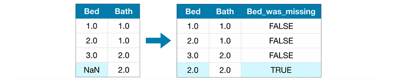
(4) Imputation + Adding Column
Sometimes when the missing values are not missed randomly. Then we may consider adding one column implying if we have a missing value in that row after imputation. This column shows the likelihood that a data point is missing.
2. Handling Outliers
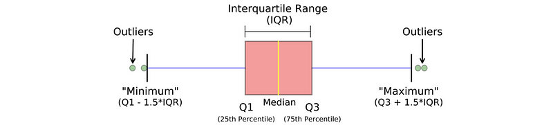
(1) The Definition Of InterQuartile Range (IQR)
The interquartile range (IQR) is a measure of statistical dispersion (e.g. one of the other examples is the standard deviation), which is the spread of the data. It is defined by,

Where,
- Q3 is the 75th percentile
- Q1 is the 25th percentile
Note that Q2 (50th percentile) is also called the median.
(2) The Definition of Outliers
An outlier is an observation that lies outside the overall pattern of distribution. There are two types of outliers.
- Normal Outlier: Outliers that can be detected within a column. It is defined mathematically as,

Note that there are many other definitions of outliers and you can find them in this paper.
- Joint Outliers: Outliers that occur when comparing relationships between two sets of data.
(3) Outlier Detection
- Histogram: The data lies outside the distribution of a feature is an outlier

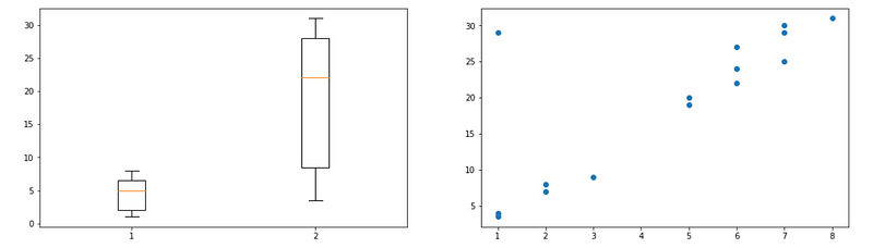
- Box Plot: The data that lies outside the minimum-maximum range is an outlier. This is the simplest way for outlier detection.
- Scatter Plot: However, the joint outliers can not be detected by the box plot because the data is still in the distribution of each column. In this case, we may think about using a scatter plot instead of a box plot for finding the outlier.
(3) Outlier Solutions
- Drop Row: A human mistake or error will definitely not be helpful for prediction. But be careful about this because we may lose some critical information.
- Imputation: Even if the outlier is confirmed to be a mistake, we may still want to take the advantage of other information in this record. So instead of dropping the row, we can impute the outlier. Common imputation methods include using the mean of a variable or utilizing a regression model to predict the missing value.
- Capping/Flooring: This is the simplest way to deal with the errors by capping the outliers with the 1st percentile or 99th percentile of the data.
- Transformation: When the outlier is not caused by mistake. For example, California has a way higher drug cost compared with other states. We can think about using the log-transformed data rather than using the data itself.
- Consider a Tree-Based Model: Trees are extremely good at handling outliers because they will shunt them to small leaves.
3. Handling Categorical Data
(1) Label Encoding
Typically, with label encoding, categorical values are replaced with a numeric value between 0 or 1 and the number of classes minus 1 or the number of classes.

The advantages of label encoding are,
- Less memory consumption because only 1 column is added
- Works well with tree-based models because tree-based models don’t take ordinal information into account while splitting
- Works well with ordinal category data
The drawbacks of label encoding are,
- Implies the order of categories (e.g. Broccoli > Chicken > Apple)
- Implies the non-existed relationship (e.g. mean(Broccoli, Apple) = Chicken)
- Can not be used with linear models
- Can not be used with neural networks
(2) One-Hot Encoding (OHE)
OHE converts each categorical value into a new categorical column and assigns a binary value of 1 or 0 to those columns. Each integer value is represented as a binary vector.

The advantages of OHE are,
- Works well with tree-based models but we commonly don’t choose it because it is very expensive
- Works well with linear models and neural networks
The drawbacks of OHE are,
- Expensive memory consumption because only # of classes of columns are added. This is also called the curse of dimensionality. We may need to apply dimensional reduction methods like PCA.
- Can not be applied to ordinal category data because we lose information
(3) Trade-off: Hash Encoding
We have discussed that label encoding is extremely good at the cost but it can not be used for linear models or neural networks. Besides, OHE is extremely good for working with linear models or neural networks, but it is not appropriate to use because we will have too many dimensions. A trade-off approach to these two methods is hash encoding. It maps each category into a vector of d dimensions, and we have,
- when
d = 1: it is equivalent to label encoding - when
d = # of classes: it is equivalent to one-hot encoding
Commonly, we can assign dimension d to a value between 3 to 5 for avoiding a high cost of encoding.
The advantages of hash encoding are,
- It is faster and memory-efficient than OHE
- It works well with linear models and neural networks
- It can work with tree-based models but again, label encoding is enough for these models
The drawbacks of hash encoding are,
- There can be a low probability of collisions because of the hash function. But the probability is very low so that it can be ignored.
- We can not interpret our features after encoding
- Feature Importance no longer works
- The dimension of the hash vector is a hyperparameter and it is hard to decide.
(4) Categorical Embeddings
An embedding is a vector representation of a categorical variable. We will take more about it in the future. This can be used for neural networks and linear models.
4. Feature Engineering
(1) Categorical Feature Engineering
- Target/Mean Encoding
Compute the mean per category for the categorical feature. For overfitting, we have to generalize this encoding by cross-validation. For avoiding zero means, we can consider applying Laplace smoothing.

- Frequency Encoding
Make a column with the frequency of each category.

- Expansion Encoding
We can create multiple variables from a high cardinality variable like strings or JSON results.
(2) Numerical Feature Engineering
- Binning Encoding
In this method, the data is first sorted and then the sorted values are distributed into a number of buckets or bins. It requires some heuristic or domain knowledge. For example, ages to generations.
- Rank/Quantile Transformation
This is a method for map values to rank or quantiles. It can smooth out the distribution and wrap out the outliers.
- Power Transformation
This is a common way of transforming data that is not normally distributed. For example, if the data is positive and right-skewed, we can use log or sqrt for transformation.
- Interaction Transformation
We can also encode interactions between variables like subtractions and addition.
5. Imbalanced Data
(1) Examples of Imbalanced Data
- Cancer Diagnosis
- Tumor Classification
- Credit Card Fraud
- Computer Version
(2) Undersampling Major Class
- Random undersampling
The simplest undersampling technique involves randomly selecting examples from the majority class and deleting them from the training dataset. This can lead to deleted useful information.
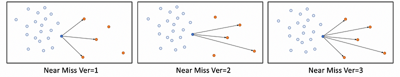
- Near miss undersampling
Select samples based on the distance of majority class examples to minority class examples. Typically, there are three methods for this technique,
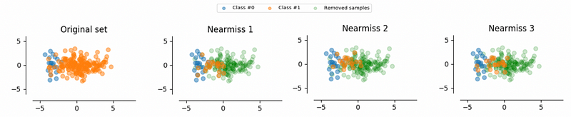
a. NearMiss-1 : Select majority class examples based on the minimum average distance to the n_neighbors closest minority class examples.
b. NearMiss-2 : Select majority class examples based on the minimum average distance to the n_neighbors furthest minority class examples.
c. NearMiss-3 : Select majority class examples based on the minimum average distance to all the minority class examples.
- Condensed Nearest Neighbors (CNN)
CNN seeks a subset of a collection of samples that results in no loss in model performance. This is implemented by enumerating the examples in the majority class and trying to classify them with a dataset starting with the minority class.
// Note: negative is major, positive is minor
Step 1: E = {positive examples}
Step 2: Loop through the whole majority dataset
Step 2-1: If we can not classify correctly by E with nearest neighbor algorithm, put data in E
Step 2-2: Else, discard the current data
Step 3: Break the loop when we traversed the whole majority set
Step 4: Return E as the balanced set
- Tomek Links Extension
We will not talk about this one in detail but this is very popular recently. Tomek defines the decision boundary where we can sample around. Note that x1 and x2 are considered to have a Tomek Link if a) the nearest neighbor of x1 is x2; 2) the nearest neighbor of x2 is x1; and 3) x1 and x2 belong to different classes. An application of Tomek Link is called One-Sided Selection,
Step 1: D = random({negative examples})
Step 2: E = {positive examples}
Step 3: Classify each x in D with E
Step 4: Move all the misclassified x into E
Step 5: If x == Tomek Links, E.remove(x)
Step 6: Return E
Step 5 removes from E all negative examples participating in Tomek Links. This removes those negative examples which are considered borderline or noisy. Remember that all positive examples are retained in the set.
- Edited Nearest Neighbor Rule (ENN)
Step 1: For x in E = {training set examples}
Step 2: NNs = x.getThreeNearestNeighbor()
Step 3: If x in major and kNN_clf(x, NNs) != x, E.remove(x)
Step 4: If x in minor and kNN_clf(x, NNs) != x, E.remove(NNs)
Step 5: Back to Step 1
Step 6: Return E
(3) Over-sampling Minor Class
- Random oversampling
Randomly duplicate examples from the minority class.
- Synthetic Minority Oversampling Technique (SMOTE)
The minority class is over-sampled by creating synthetic examples along with the line segments of k minority class nearest neighbors.
(4) Metrics for Imbalanced Data
We should not use accuracy for imbalanced data, instead, we have to consider the recall rate (sensitivity).