Intro to Machine Learning 9 | Evaluation Metrics
Intro to Machine Learning 9 | Evaluation Metrics

- Regression Metrics
(1) Mean Square Error (MSE)

The best constant function that would minimize this error is,

(2) Root Mean Square Error (RMSE)

The best constant function that would minimize this error is,
(3) R-Squared (R²)

The best constant function that would optimize this value is,

(4) Mean Absolute Error (MAE)

The best constant function that would minimize this error is,

(5) Mean Absolute Error Vs. Root Mean Square Error
- RMSE and MSE give a relatively high weight to large errors
- MAE is used as a Metric and Loss function
- Both MAE and RMSE measure average model prediction error in units of the variable of interest
- Use MAE when we have outliers
2. Classification Metrics
(1) Log Loss (Entropy)
For multi-class classification,

Especially when the number of classes = 2,

For multi-label classification,

(2) Confusion Matrix
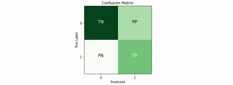
- True positive: correctly predict the positive class
- True negative: correctly predict the negative class
- False positive: wrongly predict the positive class, also called type I error
- False negative: wrongly predict the negative class, also called type II error
(3) Confusion Matrix Metrics
- Accuracy
Accuracy = TP + TN / (TP + TN + FP + FN)
- Recall / Sensitivity / True positive rate
Sensitivity = TP / (TP + FN)
- Precision
Precision = TP / (TP + FP)
- False positive rate
False positive rate = FP / (FP + TN)
- True negative rate
True negative rate = TN / (FP + TN)
- F1 score
The formula for the standard F1-score is the harmonic mean of the precision and recall.

Or,

- Fβ score: a more general case of F1 score

(4) Area Under Curve (AUC)
There are two ways of interpreting AUC. One is the area under the ROC curve or PR curve, which can also be noted as ROC-AUC or PR-AUC. Another definition is the ordering of the pairs, which is the probability the model will score a randomly chosen positive class higher than a randomly chosen negative class. For this definition, the expression should be,
AUC = # of ordered pairs / total # of pairs
The pair here is defined as positive-negative label pairs and there are in total,
Total # of pairs = # of pos label * # of neg label
A wrongly ordered pair is defined when we have the true labels ordered by the soft predictions and then count how many 1s we have in front of 0s.
0 0 0 1 0 1 1 1 ->  1 wrongly ordered pair
0 0 1 0 0 1 1 1 ->  2 wrongly ordered pair
0 0 1 0 1 0 1 1 ->  3 wrongly ordered pair
1 0 1 0 1 0 1 0 -> 10 wrongly ordered pair
1 1 1 1 0 0 0 0 -> 16 wrongly ordered pair
AUC can also be calculated as,
AUC = 1 - # of wrongly ordered pairs / total # of pairs
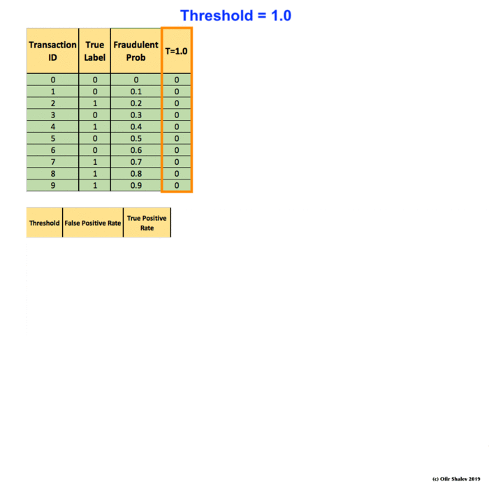
(5) Receiver Operating Characteristic (ROC)
To manually compute a ROC curve, we have to set up some thresholds and use them for hard predictions. For each threshold, we can then calculate the false positive rate and the true positive rate (recall). Finally, we should put them together on a plot and link them together. That is the ROC line we are going to have.
(6) Precision-Recall AUC (PR-AUC)
Similar to the ROC-AUC curve, if we have precision vs recall instead of recall vs false positive rate, we can generate a PR curve and the area under this curve is the PR-AUC matric.

(7) ROC-AUC (AUROC) vs PR-AUC (AUPRC)
- PR-AUC is more sensitive to the improvements for the positive class, so choose this when you care more about the positive values. Especially for the case when we have imbalanced data.
- Instead, we suggest using ROC-AUC because it cares equally about the positive and negative classes.