Java Programming 6 | Functions and Libraries
Java Programming 6 | Functions and Libraries

- Modular Programming
(1) The Definition of Libraries
A library is a set of functions.
(2) The Definition of Java Modules
A java module is a .java file. Because a java module contains sets of functions, libraries and modules are basically the same thing.
(3) The Definition of Java Functions
The java functions, which are also called the static methods, take zero or more arguments and return zero or more output values. Because Java functions are more general than mathematical functions, they may cause some side effects like bugs, exceptions, or other calls.
(4) main Function
The main function is the entrance where we start when we execute a program. Therefore, we can only have one main functions in one program and the name of this function must be main.
(5) The Definition of Scope
The scope of a variable i the code that can refer to it by name. In a Java library, a variable’s scope is the code following its declaration, in the same block.
(6) Flow of Control
In Java, OS first calls main() on java command. Then the control transfers to the function code. Then argument variables are declared and initialized with the given values and the function code is executed. Finally, control transfers back to the calling code with the return value assigned in place of the function name in the calling code.
2. Case Study of Functions: Digital Audio
(1) The Definition of Sound
Sound is the perception of the vibration of molecules.
(2) The Definition of Musical Tone
A musical tone is a steady periodic sound.
(3) The Definition of Pure Tone
A pure tone is a sinusoidal waveform.
(4) The Definition of Samples
Similar to drawing a function, the representation of a sound wave is also discrete, and it is decided by how many samples per second. This concept is called samples because it is firstly the samples we take for recording sounds. A Sony standard CD has 44,100 samples per second.
(5) StdAudio Library
- play a
wavfile
void play(String filename)
- play the given sound wave
a
void play(double[] a)
- save the soundtrack to a
wavfile
void save(String file, double[] a)
- read from a
wavfile
double[] read(String file)
(6) Example 1: Play A Note
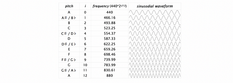
Let’s now see the simplest example for the StdAudio Library. We would like to use this library for playing a note with given seconds. We will take in two arguments, hz means the frequency of the sound, and we can have a quick reference with the following table (e.g. A = 440 Hz),
duration means how long the note lasts (a duration = 1 means 1 second). The standard we use is to have 44,100 samples per second, so we need to calculate 44,100 pieces of data per second. We need to calculate the array a based on the following formula,

Therefore, the program should be,
public class PlayNote {
   public static void main(String[] args) {
        double hz = Double.parseDouble(args[0]);
        double duration = Double.parseDouble(args[1]);
        int N = (int) (44100 * duration);
        double[] a = new double [N+1];
        for (int i = 0; i < N; i++) {
         a[i] = Math.sin(2 * Math.PI * i * hz / 44100);
        }
        StdAudio.play(a);
 }
}
We can test this program by,
$ java PlayNote 440 1
(7) Example 2: Modulized Play A Note
In the last example, our code is not modulized. To modulize the code above, we are going to create a function tone. This function takes in two arguments hz and duration, and then it outputs the sound wave sequence a. In the main function, we don’t need to realize the details about the tune function anymore, what we can do now is to focus only on the inputs and the outputs. This will bring us some benefits that we are going to talk about in the future. The program should be,
public class PlayThatNote
{
    public static double[] tone(double hz, double duration)
    {
        int N = (int) (44100 * duration);
        double[] a = new double[N+1];
        for (int i = 0; i <= N; i++)
            a[i] = Math.sin(2 * Math.PI * i * hz / 44100);
        return a;
    }
    public static void main(String[] args)
    {
        double hz = Double.parseDouble(args[0]);
        double duration = Double.parseDouble(args[1]);
        double[] a = tone(hz, duration);
        StdAudio.play(a);
    }
}
(8) Example 3: Modulized Play Für Elise
Before we start to write the next program, how about listening to the one piece of music,
Would you like to play this music with your program? Let’s have a try. In this example, we will use the PlayThatNote.tone method we have created. You can find out that one benefit of modulize the program is that we can easily reuse some functions.
The data of this music can be found at this link. And based on this data, we have to change the code a little bit. We can find out in this data file elise.txt , the notes are represented by the numbers from 0 to 12. The formula to transfer these numbers to frequencies is as follows,

The program should be,
public class PlayThatTune
{
    public static void main(String[] args)
    {
        double tempo = Double.parseDouble(args[0]);
        while (!StdIn.isEmpty())
        {
            int pitch = StdIn.readInt();
            double duration = StdIn.readDouble() * tempo;
            double hz = 440 * Math.pow(2, pitch / 12.0);
            double[] a = PlayThatNote.tone(hz, duration);
            StdAudio.play(a);
        }
        StdAudio.close();
    }
}
We can test this code by,
$ curl https://introcs.cs.princeton.edu/java/21function/elise.txt | java PlayThatTune 1
Aha, it sounds awful, right? Let’s find some ways to improve this.
(9) Example 4: Play the Chords
If we can implement chords, our music must sound better. But what is the theory of chords? Well, in conclusion producing chords means averaging waveforms. Let’s see an example. Suppose we have two sound waves a[] and b[] , then their chord will simply be the average of them c[] = a[] / 2 + b[] / 2 . Based on this theory, we can create a program that can play chords of two notes (remember that using PlayThatNote.tone saves our time),
public class PlayThatChord
{
    public static double[] avg(double[] a, double[] b)
    {
        double[] c = new double[a.length];
        for (int i = 0; i < a.length; i++)
            c[i] = a[i]/2.0 + b[i]/2.0;
        return c;
    }
    public static double[] chord(int pitch1, int pitch2, double d)
    {
        double hz1 = 440.0 * Math.pow(2, pitch1 / 12.0);
        double hz2 = 440.0 * Math.pow(2, pitch2 / 12.0);
        double[] a = PlayThatNote.tone(hz1, d);
        double[] b = PlayThatNote.tone(hz2, d);
        return avg(a, b);
    }
    public static void main(String[] args)
    {
        int pitch1 = Integer.parseInt(args[0]);
        int pitch2 = Integer.parseInt(args[1]);
        double duration = Double.parseDouble(args[2]);
        double[] a = chord(pitch1, pitch2, duration);
        StdAudio.play(a);
    }
}
And we can test it by,
% java PlayThatChord 0 3 1.0
% java PlayThatChord 0 12 1.0
(10) Example 5: Play Für Elise with Harmonics
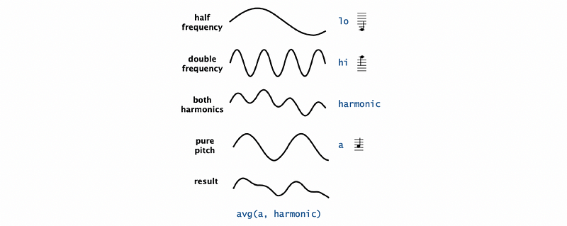
By adding harmonics to PlayThatTune , we can produce a more realistic sound. The algorithm that we are going to use is firstly averaging the half frequency lo and the double frequency hi for the current pitch, and what we generate is so-called both harmonics. Then we will average these harmonics with the pure pitch a, which will create our final result. The algorithm method is called note and it will be as follows,
public static double[] note(int pitch, double duration) {
    double hz = 440.0 * Math.pow(2, pitch / 12.0);
    double[] a  = PlayThatNote.tone(hz, duration);
    double[] hi = PlayThatNote.tone(2*hz, duration);
    double[] lo = PlayThatNote.tone(hz/2, duration);
    double[] h  = sum(hi, lo, 0.5, 0.5);
    return sum(a, h, 0.5, 0.5);
}
What’s more, we also need to work out a function for averaging the pitches. This function should be called sum and it takes 4 arguments. Of course, two of them are the arraies of these two pitches. We also have two other arguments, awt and bwt , which simply means the weight of pitch a and pitch b. These values should be subject to the rule of awt + bwt = 1.
The function sum should be,
public static double[] sum(double[] a, double[] b, double awt, double bwt) {
    assert a.length == b.length;
    double[] c = new double[a.length];
    for (int i = 0; i < a.length; i++) {
        c[i] = a[i]*awt + b[i]*bwt;
    }
    return c;
}
So in general, the program that we can play a tune with harmonics is,
public class PlayThatTuneDeluxe {
    public static double[] sum(double[] a, double[] b, double awt, double bwt) {
        assert a.length == b.length;
        double[] c = new double[a.length];
        for (int i = 0; i < a.length; i++) {
            c[i] = a[i]*awt + b[i]*bwt;
        }
        return c;
    }
    public static double[] note(int pitch, double duration) {
        double hz = 440.0 * Math.pow(2, pitch / 12.0);
        double[] a  = PlayThatNote.tone(hz, duration);
        double[] hi = PlayThatNote.tone(2*hz, duration);
        double[] lo = PlayThatNote.tone(hz/2, duration);
        double[] h  = sum(hi, lo, 0.5, 0.5);
        return sum(a, h, 0.5, 0.5);
    }
    public static void main(String[] args) {
        while (!StdIn.isEmpty()) {
            int pitch = StdIn.readInt();
            double duration = StdIn.readDouble();
            double[] a = note(pitch, duration);
            StdAudio.play(a);
        }
    }
}
We can retry the music and see if it sounds better this time,
$ curl https://introcs.cs.princeton.edu/java/21function/elise.txt | java PlayThatTuneDeluxe 1.5
Or we can also try something new,
$ curl https://introcs.cs.princeton.edu/java/21function/entertainer.txt | java PlayThatTuneDeluxe 1.5
3. Application of Functions: Gaussian Distribution
In this part, we will write a bunch of functions that can be used for Gaussian distribution. As what we have talked about in the other series, the Gaussian distribution is a mathematical model that has been used successfully for centuries. It gives useful conclusions for engineering and experimenting.
The standard Gaussian distribution should be,

And a more general form with the standard deviation σ and the mean value μ is,

Now let’s write our first function, the standard PDF for Gaussian distribution in the Gaussian class,
public class Gaussian
{
    public static double pdf(double x)
    {
        return Math.exp(-x*x / 2) / Math.sqrt(2 * Math.PI);
    }
}
Now, if we want to add a more general PDF with μ and σ, what can we do? Can we use the same function name pdf? The answer to this question is yes. Functions and libraries provide an easy way for any user to extend the Java system. Java functions with different arguments are different even if their names match. So the general function is,
public class Gaussian
{
    public static double pdf(double x)
    {
        return Math.exp(-x*x / 2) / Math.sqrt(2 * Math.PI);
    }
    public static double pdf(double x, double mu, double sigma)
    {
        return pdf((x - mu) / sigma) / sigma;
    }
}
Another function we have to implement is the Gaussian cumulative distribution function. It is actually the integration of the Gaussian PDF. However, due to the limitations of mathematics, we can not work out the precise result of this integration. For example, the standard form of its standard CDF should be,

Typically, we get the result of this integration by referring to a table. However, another way to get the result by hand easily is to use the Taylor series. The formula of the Taylor series for the Gaussian CDF is,

When z is in the scope of (-8, 8), the sum of terms in this series is convergence. However, when z > 8 or z < -8, the result of this series will be 1 and 0, respectively. When this sequence converges, based on the feature of a double value, we can finally find a time when sum + term == sum. And we are going to use a loop to get the value for some of the terms at this time. The program should be,
public static double cdf(double z)
{
    if (z < -8.0) return 0.0;
    if (z > 8.0) return 1.0;
    double sum = 0.0, term = z;
    for (int i = 3; sum + term != sum; i += 2)
    {
        sum = sum + term;
        term = term * z * z / i;
    }
    return 0.5 + sum * pdf(z);
}
public static double cdf(double z, double mu, double sigma)
{ return cdf((z - mu) / sigma); }
So finally, let’s write the main function. The main function takes in three arguments z , mu , and sigma . And it will print the value of the Gaussian CDF. Therefore, the code of the main function should be,
public static void main(String[] args)
{
    double z = Double.parseDouble(args[0]);
    double mu = Double.parseDouble(args[1]);
    double sigma = Double.parseDouble(args[2]);
    StdOut.println(cdf(z, mu, sigma));
}
4. Modular Programming
(1) The Definition of Signatures
The signature of a function in Java includes,
- parameters and their data types
- a return value and its data type
- exceptions that might be thrown or passed back
- information about the availability of the method in an object-oriented program (such as the keywords
public,static, orprototype).
Functions with different signatures will be treated as different functions even though their function names match.
(2) The Definition of Application Programming Interface (API)
The API is a list that defines the function signatures and describes methods. For example, the API for Gaussian class is,
public static double pdf(double x)
public static double pdf(double x, double mu, double sigma)
public static double cdf(double z)
public static double cdf(double z, double mu, double sigma)
(3) StdRandom Library APIs
The standard random library StdRandom is base on the Math.random() function. It can be used for generating random values based on various distributions.
- generate random integers between
0toN-1
int uniform(int N)
- generate random reals between
loandhi
double uniform(double lo, double hi)
- generate boolean values based on the Bernoulli distribution
boolean bernoulli(double p)
- generate random reals based on standard Gaussian distribution
double gaussian()
- generate random reals based on Gaussian distribution with mean
mand standard deviations
double gaussian(double m, double s)
(4) Example 1: 2D Gaussian Distribution
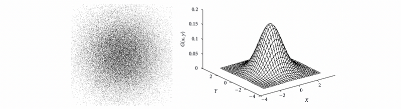
Now, let’s see an application. Suppose we have an X-Y coordinate plane and the points we are going to draw in this plane follows the Gaussian Distribution both on the X-axis and the Y-axis. Then, the program should be as follows,
public class RandomPoints
{
    public static void main(String[] args)
    {
        int N = Integer.parseInt(args[0]);
        for (int i = 0; i < N; i++)
        {
            double x = StdRandom.gaussian(0.5, 0.2);
            double y = StdRandom.gaussian(0.5, 0.2);
            StdDraw.point(x, y);
        }
    }
}
(5) StdStats Library APIs
The StdStats library is implemented for computing statistics on arrays of real numbers. Common methods are,
- get the largest value
double max(double[] a)
- get the smallest value
double min(double[] a)
- get the mean value
double mean(double[] a)
- get the sample variance
double var(double[] a)
- get the standard deviation
double stddev(double[] a)
- get the median value
double median(double[] a)
- plot all the points at (i, a[i])
void plotPoints(double[] a)
- plot lines connecting points at (i, a[i])
void plotLines(double[] a)
- plot bars to points at (i, a[i])
void plotBars(double[] a)
(6) Example 2: Bernoulli Trials and Central limit theorem
Now, let’s see an example of the Bernoulli trials, and let’s see if the result of this experiment follows the Gaussian distribution. The question is as follows, suppose we have a coin and we would like to flip it for N times and see how many heads we have. We are going to repeat this trial for trials times, and finally draw a bar plot of experimental result. We are also going to draw the theoretical curve of the Gaussian distribution and see if these two results match. The program should be,
public class Bernoulli
{
    public static int binomial(int N)
    {
        int heads = 0;
        for (int j = 0; j < N; j++)
            if (StdRandom.bernoulli(0.5))
                heads++;
        return heads;
    }
    public static void main(String[] args)
    {
        int N = Integer.parseInt(args[0]);
        int trials = Integer.parseInt(args[1]);
        int[] freq = new int[N+1];
        for (int t = 0; t < trials; t++)
            freq[binomial(N)]++;
        double[] normalized = new double[N+1];
        for (int i = 0; i <= N; i++)
            normalized[i] = (double) freq[i] / trials;
        StdStats.plotBars(normalized);
        double mean = N / 2.0;
        double stddev = Math.sqrt(N) / 2.0;
        double[] phi = new double[N+1];
        for (int i = 0; i <= N; i++)
            phi[i] = Gaussian.pdf(i, mean, stddev);
        StdStats.plotLines(phi);
    }
}
And the output should be,
$ java Bernoulli 20 10000

This is one special case of the central limit theorem (or CLT), and it states the fact that, in many situations, when independent random variables are added, their properly normalized sum tends toward a normal distribution even if the original variables themselves are not normally distributed.