Linear Algebra 2 | Various Matrix, Matrix Equations, Gaussian Elimination, and Matrix…
Linear Algebra 2 | Various Matrics, Matrix Equations, Gaussian Elimination, and Matrix Multiplication

- Matrix
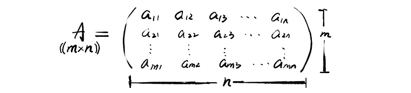
(1) Definition of Matrix and Entry: A matrix is a rectangular array. The places in the matrix where the numbers are is called entries (i.e. horizontal entries and vertical entries).
- the greyscale image is a matrix
- a mass dataset
- etc…
(2) The shape of the Matrix
The shape of a matrix is the # (number) of the rows times the # of the columns. For example, the following matrix A has a shape of 2 × 3 and the notation of the shape is A((2 × 3)).

(3) Square Matrix
When the # of the rows of a matrix equals the # of the columns of it, this matrix is thought to be a square matrix. For example, the following matrix B is considered to be a square matrix.

(4) Project from ℝⁿ to ℝᵐ (x: ℝⁿ → ℝᵐ )
Suppose we have a vector x ∈ℝⁿ and we want to project it to vector space ℝᵐ, so what we can do here is to construct a projection matrix A which has a shape of m x n. In this specific case, we can think of matrix A as a function ( mapping/transformation function) from x: ℝⁿ — A→ ℝᵐ. For example,
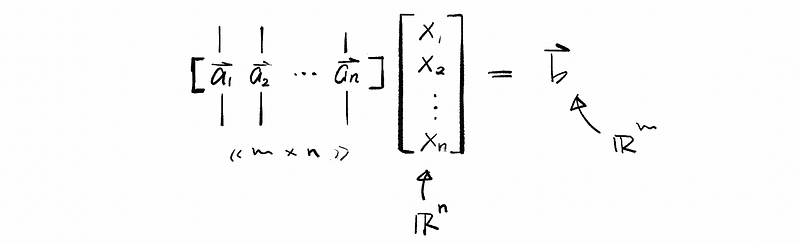
If we treat each column in matrix A as a vector, such as a1, a2, a3, …, an, we can write this matrix in a way that is similar to a vector. For example,

So that if we use matrix A times vector x, we are going to calculate a new vector in the vector space ℝᵐ. So what are we going to say here is quite simple that the vector b ∈ℝᵐ which we worked out just now is the A-transformation of vector x.
Here, we have defined that vector b ∈ ℝᵐ is the result of A times x. So the vector b is a linear combination on the columns of A that we get by using the components of x as weights.

Another perspective is that the i-th component of vector b (aka. bi) could be treated as the dot product of the vector ai and the vector x.

(5) Matrix Equation
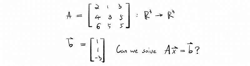
Suppose we have matrix A((m × n)): ℝⁿ → ℝᵐ, can we find a vector x in ℝⁿ so that A · x = b (for some b)? (Or the question could be that, what linear combination of A will give us b (if any)?) The answer is yes and given matrix A and vector b, we can solve this matrix equation A · x = b. For example,
The solution is, first of all, we have to create a linear combination based on what we have said previously.
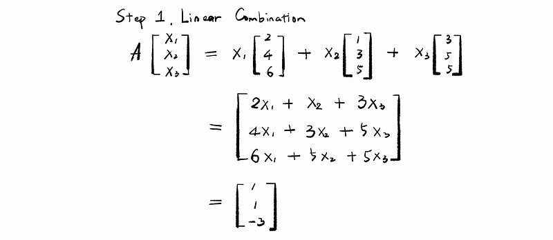
Secondly, we construct a system of equations in three variables in order to calculate x1, x2, and x3.
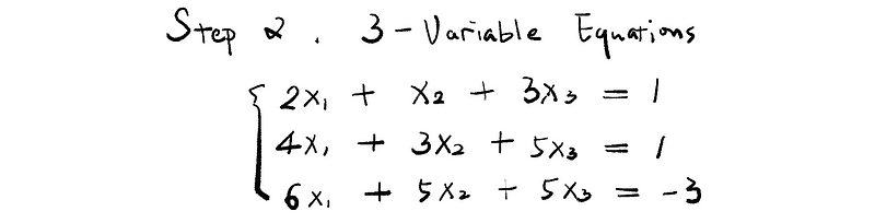
Thirdly, we conduct the Back Substitution algorithm to get x1, x2, and x3.
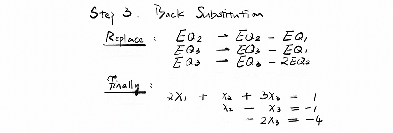
Fourthly, we can solve the system as,

Finally, we have got our conclusion,

(6) Augmented Matrix
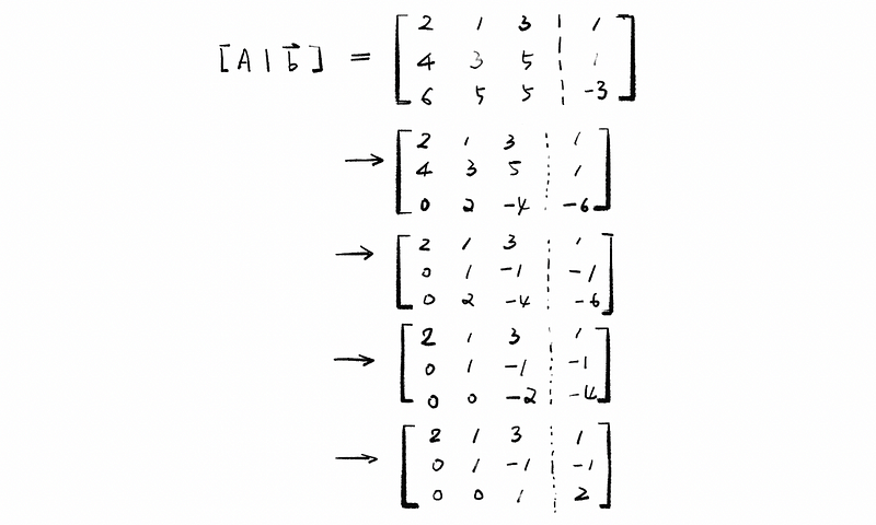
In the previous case that we can solve the matrix equation A · x = b. Now we define the matrix [ A | b ] as an augmented matrix. This is partly because each row of [ A | b ] could do algorithms of the matrix. Well, from the perspective of equations, matrix A could also be reckoned as the coefficient matrix. For example,

(7) Row Operations
The row operations of a matrix follow the following steps:
- multiply row by a number
- add a multiple of one row to another row
- change the rows
(8) Gaussian Elimination
The definition of elimination is to apply these row operations until we get to an upper triangular form matrix.
Gaussian elimination, which is also known as row reduction, is used to solve a system of linear equations. It is quite similar to what we have already done there. For example, we can use Gaussian elimination for the previous augmented matrix,
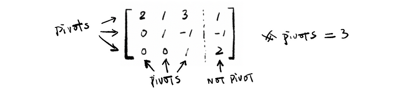
(9) Pivots
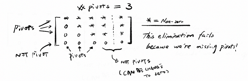
The non-zero entries that we use in elimination to eliminate below are called pivots. Elimination fails when we are missing pivots. So the number of pivots should equal the number of unknown variables if we can solve the equation. For example,
And for the previous case, we have,
(10) Upper Matrix
The upper matrix is also called the upper triangular matrix with the down-left element of the matrix all equal to zero. For example,

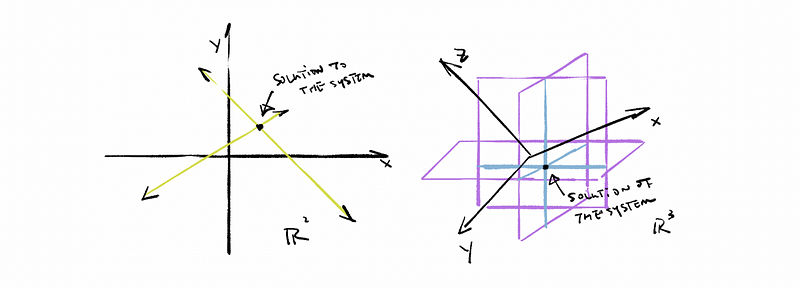
(11) The Geometry of the Linear Equations
Geometrically, the linear equations in ℝ² are lines and the linear equations in ℝ³ are planes. The solution of the system is the counterpoint of these lines or planes.
(11) Linear Transformation: Easy Algebra Rectifications
Suppose we have vector spaces V and W along with the transformation matrix (aka. mapping matrix) A. So the rule A: V → W is called a linear transformation. For any of the vectors x ∈V and y ∈ V, given constant c as a scalar, x and y satisfy two conditions:
- Condition 1: Additivity

- Condition 2: Homogeneity

(12) Two Times Transformation
Suppose that A is an m × n mapping matrix from vector space V: ℝⁿ to vector space W: ℝᵐ, and B is an n × p mapping matrix from vector space P: ℝᵖ to vector space V: ℝⁿ. Given that vector x ∈ℝᵖ. So that we can have a relationship of x: ℝᵖ → ℝⁿ → ℝᵐ. The graph is as follows,
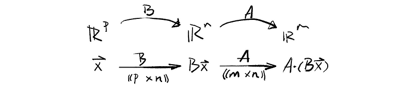
We would like to prove the equation that A(Bx) = (AB)x, so how to prove it?
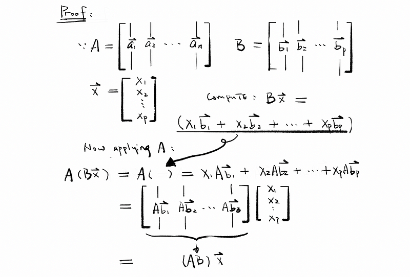
As a result, we can conclude that given transformation matrix AB, we can transform vector x: ℝᵖ → ℝᵐ.
(13) Matrix Multiplication
Now, look at the entry in the i-th row and j-th column of AB, as (AB)ij. So we could have,
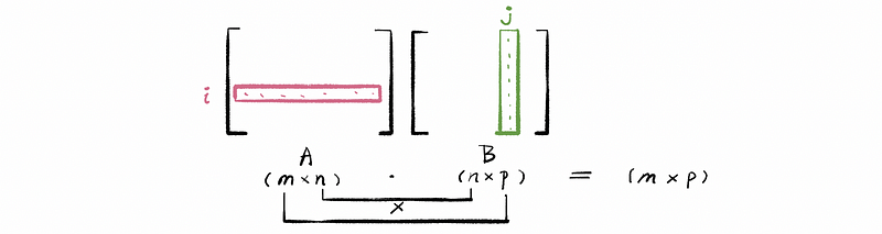
Let’s take Abj, which is also the j-th column of the final result, we could then have the formula (i-th row of A) ⋅ bj:

(14) Properties fo the Matrix
- AB ≠ BA
- A² = 0 not ⇒ A = 0, counterexample:

- A(BC) = (AB)C
- A(B+C) = AB + AC, while B and C should be in the same size
- (B+C)A = BA + CA, while B and C should be in the same size
- (r + s)A = rA + sA
(15) Identity Matrix
The square matrix ((n x n)) with 1 on the diagonal and 0 on elsewhere.

(16) Inverse Matrix
Given a square matrix A((n x n)), then the inverse of A (if it exists) is the inverse matrix. Where,

(17) Transpose Matrix
The matrix we get by interchanging rows and columns of A.

(18) Properties of Inverse Matrix and Transpose Matrix