Linear Algebra 3 | Inverse Matrix, Elimination Matrix, LU Factorization, and Permutation Matrix

Linear Algebra 3 | Infinity Solutions, Inverse Matrix, Elimination Matrix, LU Matrix Factorization, Permutation Matrix, and Subspace

1. Solving Equation System with Infinity Solutions

(1) Recall: Solve An Equation

Let’s solve the following equation system Ax = b as follows,

Plan:

Perform row operations until the system is upper triangular-ish.

Ans:

By row reduction,

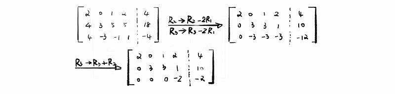
For the final matrix after the row reduction, we can then have,

We have now discovered that this equation system has three pivots and four unknown variables, which means that it will have infinite solutions. How can we solve a system like that? Well, let’s remain this as a question and after we finish the following discussions, we are going to come back to solve this system.

(2) The Definition of Entry

All the elements in a matrix are so-called entries. The first non-zero entry in a row is called the leading entry. All entries below a leading entry are 0.

(3) Recall: The Definition of Pivot

The pivot (aka. pivot element) is a specific element in a matrix. After the algorithm of Gaussian elimination (aka. row reduction) on a matrix, the leading entry of each line is called a pivot element. It is clear that all the pivots should be the leading entry in the matrix but however, the leading entry doesn’t have to be a pivot if the matrix is not operated by row reductions.

(4) Pivot Column

The columns with pivot are called pivot columns.

(5) Free Variables

The columns without pivot are called free variables.

(6) Row Echelon Form (REF) of Upper-Triangular

• Any zero rows are below any non-zero rows
• The leading entry (1st non zero entry) in any row is the right of the leading entry in the row above
• All entries in a column below a leading entry are 0

(7) Reduced Row Echelon Form (RREF)

If we have the row echelon form of a matrix and we continue eliminating the above pivots and sealing pivots to be 1, it gets us to the reduced row echelon form. To mention that the reduced row echelon form inherits all the properties and it has two extra properties as follows,

• All entries in a column above a pivot are 0
• All pivots should be set to 1

(8) Solve the Equation System with Infinity Solutions

For all the free variables in a matrix, we assign them with an abstract constant, for example, c. After that, we can then solve the equation system in a simple way with the pivot columns being represented by the expressions with c.

Thus, we come back to solve our first equation system, the matrix after row reduction is represented as,

then, because column #1, #2, and #4 are pivot columns and column #3 is a free variable. So that we assign constant c to x3 by,

then, by back substitution,

then,

then,

thus, the solution is,

given constant c ∈ ℝ.

(9) A Specific Solution of System with Infinity Solutions

We have already worked out the expression of the infinity solutions of the given equation system. Now if we assign c = 0, we can then have the solution of Ax = b as,

this is one of the easiest specific solutions that we could solve in this case.

(10) The Definition of Non-trivial Solution with Ax = 0

If we note our solution as s + ct, so the vectors s and t satisfy s, t∈ℝ⁴. By the previous discussion, we have known that s is our specific solution and then As = b. Based on the general solution, it is clear that As + cAt = b. As a result, we can derive that cAt = 0.

If c ≠ 0, the expression of cAt = 0 is also sufficed, so we can then have the conclusion that,

In our example above, we can then have,

Here we call the vector t non-trivial solution. Generally, if an echelon form of A has a free variable then there will be a non-trivial solution to Ax = 0.

(11) The Definition of Trivial Solution with Ax = 0

The definition of a trivial solution is much easier. Let’s suppose that if we have to solve the equation Ax = 0, the most direct solution is when

This is called the trivial solution of Ax = 0.

(12) Another Way to Solve an Equation System

According to our previous solution in the first example, it is quite interesting to find out that, in the special solution s, the free variable x3 is assigned to 0, while in the non-trivial solution t, the free variable x3 is assigned to 1.

In conclusion, there is only one special solution for a system and we can calculate it by assigning x3 = 0 in the equation Ax = b. However, there may be serval non-trivial solutions (the number of them is based on the number of free variables) and we can calculate them by assigning each of the free variables to 0 in the equation Ax = 0. The solution is a linear combination of these non-trivial solutions.

For example, 2- free variables means that solutions to Ax = 0 are given by linear combinations of these two vectors.

(13) Homogenous System

Basically, suppose we have a bunch of linear equations with variables multiplied by coefficients on the left-hand side and with all zeros on the right-hand side. We call the system composed of those equations homogenous system. It is considered that the homogenous system should be in the form of,

(14) Solving a Homogeneous System with Two Free Variables

Suppose we have a 3 × 5 homogeneous system,

and let’s solve it in the way of using the non-trivial solutions. This can be a little bit tricky in this case because, in a homogenous system, we don’t have to think about the special solution. The reason for this is that the special solution will be equal to zero in this case. Therefore, we can eliminate it from the general solution.

Ans:

Suppose we have two free variables x2 and x3, and also, we have two constant numbers c ∈ℝ and d ∈ℝ. By back substitution, we have,

then, we can find out that there are two free variables in this system,

then, firstly, we assign x2 = 1 and x3 = 0,

so the first non-trivial solution is,

then, secondly, we assign x2 = 0 and x3 = 1, then,

so the second non-trivial solution is,

So the general solution is,

2. Solving the Inverse Matrix

(1) The Definition of Span

Give a set of vectors {v1, v2, …, vk}, the span of this set of vectors is the set of all linear combinations of the vectors in the set. It is notated by span{v1, v2, …, vk}. For example, the solutions to Ax = 0 in the last example above is:

(2) General Solution for a Linear Equation System

Generally speaking, for all linear equation systems satisfying Ax = b, where A is our coefficient matrix, x is the vector of unknown variables and b is the vectors of all the constant terms (RHS form). Then all solutions are of the form:

where,

and,

(3) Recall: The Definition of Inverse Matrix

Let A be an n × n square matrix, then we talked about the inverse of A. If it exists, as the matrix X, so that,

(4) Calculation of Inverse Matrix

Finding matrix X is,

then,

By definition of the inverse matrix,

Then, we can have the vector equation system,

Write it in the form of the augmented matrix,

then,

However, if we write another augmented matrix as,

we can then have the relationship as,

So that it is quite clear to see that the solution matrix X suffices both of these two equation systems. Regarding the solution matrix X as a transformation matrix X: ℝⁿ → ℝⁿ. Then we can have the transformation as,

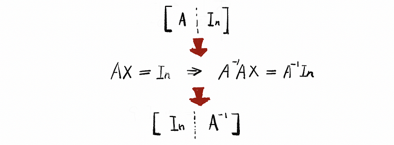
When we come back to the previous augmented matrix above, we can have,

then if we solve solution matrix X of the vector equation AX = In, we can calculate the inverse of matrix A by transforming the identity matrix In with transformation matrix X. An easier way to achieve the same result is to do row operations to the augmented matrix of AX = In, and then when the left part of this augmented matrix equals identity matrix In, the right part of this augmented matrix will be the inverse of the matrix A.

(5) Singular Matrix (aka. Non-Invertible Matrix) and Non-Singular Matrix (aka. Invertible Matrix)

If a matrix A can be inverse, which represents its RREF equals an identity matrix, then the matrix A is called a non-singular matrix (or invertible matrix). However, if the matrix A can not be inverse, which represents its RREF does not equal an identity matrix, then the matrix A is called a singular matrix (or non-invertible matrix).

(6) The Condition for Invertible Matrix

In the previous discussion, we can find out that it is sufficient for the matrix A to have an inverse matrix only if we can find a transformation matrix X that satisfies,

which to say in another way is that we can do row operations to the matrix A and then transform it into an identity matrix. As we have learned that the reduced row echelon form (RREF) for matrix A equals the identity matrix if A can be transformed into the identity matrix. So that we can check the following determinate to see whether A is a matrix that can be inverted.

(7) The Determinant of Invertible Matrix (2 × 2)

Suppose we have a matrix A as

with a, b, c, d ∈ℝ, then if we assume that A is an invertible matrix, what is the determinant of this invertible matrix?

Thus, we have,

So in conclusion, if ad = bc, there is not an inverse of matrix A, then A is an invertible matrix. Thus, the determinant is,

3. Elimination Matrix and LU Matrix Factorization

(1) Elimination Matrix: a useful tool for the solving system (can be viewed as another form of Gaussian Eliminations)

Keep in mind that elimination can be thought of as matrix multiplications. We use E to represent an elimination matrix.

Suppose that we can find a matrix A that after row reductions of this matrix, we can eliminate it to matrix B. It is the same way of saying we can find a transformation matrix E: ℝⁿ → ℝⁿ that satisfies EA = B. This transformation matrix E is called an elimination matrix. Thus, any row operations could be transferred to an elimination using the following template of elimination matrix,

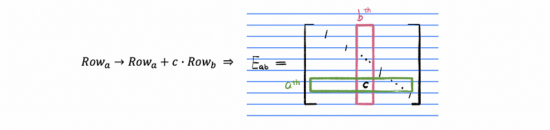
In general, the elimination matrix is an identity matrix with the entry in the a-th row and the b-th column equals the multiplier c.

(2) The Inverse of the Elimination Matrix

It is clear that the reduced row echelon form of any given matrix is the identity matrix. This is because the inverse operation of the rows could transfer an elimination matrix back to the identity matrix. So any elimination matrix is supposed to be a invertible matrix.

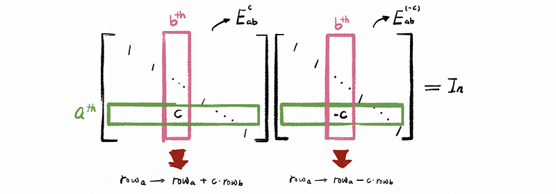
By definition of the inverse transformation, we can have the equation,

And because only inverse row operations could be treated as no change in the original matrix, so we can draw a clear conclusion that the inverse matrix transformation of the elimination matrix must have the opposite value of the entry in the a-th row and the b-th column, which, in the last example, equals c.

(3) Lower-Triangular Matrix

Recall that we have talked about the upper-triangular matrix, and similarly, the lower-triangular matrix has the form of,

(4) An Interesting Fact: Products of (Inverse) Elimination Matrix Must Be a Lower-Triangular Matrix

We have a nice fact is that the entries of the inverse row-operation matrics populate in a lower L without changing. This is because when we do row reduction (aka. back substitution, or Gaussian Elimination), we must have to do calculations of two rows and then use the result to change the row below.

This gives us a result that in the operation of row reductions of

we always have the inequation that a > b. So for any products of the elimination matrix, we can finally have a lower-triangular matrix.

(5) LU Matrix Factorization

Suppose that after n-row operations, matrix A is then transformed into row echelon form. We can write this equation as,

We have already known that the row echelon form of A is an upper-triangular matrix. If we use U to represent the upper-triangular matrix, we can then have,

then, by multiply the inverse of the elimination matrics,

by the fact that any products of (Inverse) elimination matrix must be a lower-triangular matrix, we can then use L to represent the upper-triangular matrix as,

thence, we have factorized A to the product of an upper-triangular matrix U and a lower-triangular matrix L. This is called the LU matrix factorization.

(6) A Third Way of Solving An Equation System: By Forward Substitution and Back Substitution (Application of LU factorization)

Let’s go back to our first example and we want to solve the system Ax = b. By LU factorization, we can then factorize A to LU, so then what we have to solve is the system LUx = b. We note that Ux = y, so then we are going to follow the following steps.

• Step 1: Do Forward Substitution of A and transfer it to a lower-triangular matrix, which can be easy.

• Step 2: Solve the system Ly = b.
• Step 3: Do Back Substitution of A and transfer it to an upper-triangular matrix, which can be easy as well.

• Step 4: Solve the system Ux = y.

4. Permutation Matrix

(1) Permutation Matrix

Sometimes, we have to swap the rows of a matrix. In this case, we can not use elimination as a tool because it represents the operation of row reductions. Thus, in this case, we use the permutation matrix to swap the rows in a matrix. It is notated by P.

The permutation matrix equals to swap two rows of an identity matrix. For example, suppose that we have an n-square matrix A and we would like to swap the a-th row and the b-th row of this matrix, what we can do to construct P is to swap the a-th row and the b-th row of an n-dimension identity matrix.

(2) Exchange Matrix

The exchange matrix is a particular permutation matrix, with all 1s residing the counterdiagonal and other entries being assigned as 0. It is used to get the transpose of a given matrix. For Example, an n-dimension exchange matrix should be like,

5. Subspace

A subspace of a vector space is a subset that itself a vector space. In practice, suppose we say V is a vector space (like ℝⁿ), and if W ⊆ V ( W is a subset of V ), then the two provided condition of W is a subspace satisfy:

• Condition #1

• Condition #2

A simple checker: note that when in condition #2, if c = 0, we must have 0∈W. So if 0 is not in W, then W can not be a vector space.