Linear Algebra 10 | Difference Equation and Stochastic Matrix
Linear Algebra 10 | Difference Equation and Stochastic Matrix

- Difference Equation
(1) The Definition of the Difference Equation
A difference equation is an equation of the form,

where,
- vt is the state of time t
- vt+1 is the state of time t + 1
- A is the change in a certain time period (each period = 1)
(2) Difference Equation After N Time Periods
The result of the state after time N is,

where we call,
- v0 is the original state
By observing this expression, we can know that the long-term behavior of a difference equation is an eigenvalue problem.
2. First Example: Weather Forecast
Suppose we want to have a picnic tomorrow and we are not sure if there’s going to be cloudy or sunny. Based on the statistic data from the scientists, there is a 20% chance to be sunny tomorrow if today is cloudy, while there’s an 80% chance to be cloudy tomorrow if today is cloudy. What’s more, if today is sunny, there will be a 30% chance to be cloudy tomorrow and there will be a 70% chance to be sunny tomorrow. We can draw a diagram as follows,

Now we suppose the original state is that the probability of being sunny tomorrow is equal to the probability of being cloudy tomorrow. This is to say,

We can write the difference equation as,

this is equivalent to,

So the state of whether after N days should be,

(1) What is the state after 100 days?
Run this code, and this will give us,
[0.6 0.4]
(2) What is the state after 1,000 days?
Run this code, and this will give us,
[0.6 0.4]
(3) What if we start with a random original? Will the stable state change?
Run this code, and this will give us,
[0.6 0.4]
Therefore, it is quite clear that when N is big enough, we can reach a stable state and this state is not related to the original state.
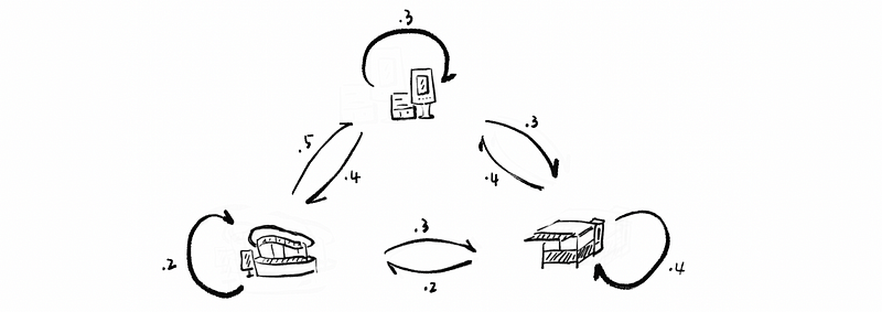
2. Second Example: RedBox Kiosks
Suppose RedBox has three kiosks in San Francisco where you can rent movies. After renting, you can return the movie to any of these three kiosks. Suppose people randomly return the movies to these three kiosks and We can draw a diagram as follows,
Now we suppose each of these three kiosks has 90 movies for renting, so our original state should be,

We can then write the difference equation as,

this is equivalent to,

also, state of time N is,

(1) What is the state after 100 renting periods?
Run this code, and this will give us,
[105. 90. 75.]
(2) What is the state after 1000 renting periods?
Run this code, and this will give us,
[105. 90. 75.]
(3) What if we start with a random original with a total of 270 movies? Will the stable state change?
Run this code, and this will give us,
[105. 90. 75.]
3. Third Example: Rabbit Population
In a population of rabbits,
- half of the newborn rabbits survive their first year;
- of those, half survive their second year;
- the maximum life span is three years;
- rabbits produce 0, 6, 8 rabbits in their first, second, and third years, respectively.
then, we can write the difference equation as,

this is also,

Start with x0=100, y0=59, z0=17, then,
(1) What is the proportion of the state after 100 years?
Run this code, and this will give us,
[0.76190476 0.19047619 0.04761905]
(2) What is the proportion of the state after 1000 years?
Run this code, and this will give us,
[0.76190476 0.19047619 0.04761905]
(3) What if we start with a random proportion (equal or less than 100 for each generation)? Will the stable proportion of the state change?
Run this code, and this will give us,
[0.76190476 0.19047619 0.04761905]
(4) What if we have a randomly generalized difference equation? Will there be a stable proportion of the state?
Run this code, we will then get three same results as expected (maybe different here because all things are randomly generated),
[0.42417225 0.2592308  0.31659696]
[0.42417225 0.2592308  0.31659696]
[0.42417225 0.2592308  0.31659696]
4. Stochastic Matrix
(1) The Definition of Stochastic Matrix
If the entries in each column sum to 1, then the matrix A is a stochastic matrix.
(2) Properties of the Stochastic Matrix
For any stochastic matrix, there are two important properties,
- λ = 1 must be an eigenvalue
- |λ| ≤ 1 for any eigenvalue
(3) Reasons for the Stable States in Example 1 & 2
Based on the eigendecomposition, we have,

then,

then,

by properties of the stochastic matrix,

because we also have |λ| ≤ 1 for any eigenvalue,

then,

thus,

therefore, when k is big enough (in our cases we used 100 and 1,000), we have,

Because this is not related to k, so a large enough k allows us to find a stable state.
(4) Reasons for the Stable Proportion of States in Example 3
In example 3, things are a little bit different because we didn’t use the stochastic matrix in the difference equation. We still can find a relationship that satisfies,

this is also to say that,

In this case, we also have,

By doing proportion in the last step, is equivalent to normalizing the matrix above, which is then,

so when k is large enough, we can also have that,
Therefore, we can also reach a stable proportion of state when k is large enough.