Linear Algebra 11 | Graph Theory Fundamentals, Random Walk Problem, Laplacian Matrix, and PageRank
Linear Algebra 11 | Graph Theory Fundamentals, Random Walk Problem, Laplacian Matrix, and Google’s Pagerank Algorithm

- Fundamental of Graphs
(1) The Definition of Vertex (aka. Node)
The vertex is a point where multiple lines meet, it is also known as the node.

(2) The Definition of Edge
The line that connects two vertices is called the edge.

If there are more than one edges connecting two vertices, then these edges are called parallel edges.

(3) The Definition of Graph
As discussed in the previous section, the graph is a combination of vertices (nodes) and edges. G = (V, E) where V represents the set of all vertices and E represents the set of all edges of the graph.

(4) The Definition of Degree
The number of edges connected to a vertex is called the degree of this vertex. It is noted as deg(vertex). For example, in the graph above, the degree of node 1 is 2, and the degree of node 2 is 3.
(5) The Adjacency Matrix of a Graph
To some extent, a graph is also a matrix. Suppose we have got a graph G with n nodes, then it can be written as an n × n matrix if it satisfies,

This is called the adjacency matrix of the graph G.
(6) The Definition of the Null Graph
For a given graph G = (V, E), if E = ∅, then this graph is called a null graph.

The adjacency matrix of a null graph is a null matrix with all the entities in it equals zero.

(7) The Definition of the Non-Directed Graph
The non-directed graphs are the graphs that have edges, but these edges do not have any particular direction.

It is quite clear that the adjacency matrix form of a non-directed graph must be a symmetric matrix because the edge that connecting node i to node j must connect node j with node i.
(8) The Definition of the Directed Graph
When the edges of a graph have a specific direction, they are called directed graphs.
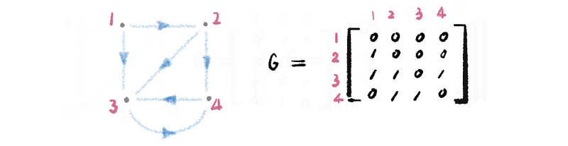
The adjacency matrix of a directed graph must be asymmetric, because if the matrix of a directed graph is a symmetric matrix, then it turns out to be a non-directed graph instead of a directed graph.
(9) The Definition of the Disconnected Graph
Starting from one point, if we have unreachable vertex(s), i.e., a path does not exist between every pair of vertices, then this graph is a disconnected graph.
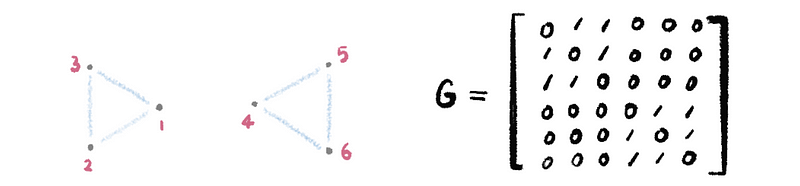
The adjacency matrix of this kind of graph is quite interesting because we have the upper right partial matrix and the lower-left partial matrix equals the null matrix (or zero) if the nodes are ordered by the order of the clusters.

(10) The Definition of the Connected Graph
Starting from one point, when there is no unreachable vertex(s), then this graph is a connected graph. For example,

(11) The Inner Degree and The Outer Degree
In a directed graph, the inner degree of a vertex equals the number of edges pointing to this vertex, while the outer degree of a vertex equals the number of edges pointing out of this vertex. For example, the following vertex has an inner degree equal to 4 and an outer degree equal to 5.

2. The Random Walk Problem
(1) Difference Equation of the Random Walk Problem
Recalling the last section when we talked about the weather forecast problem, the diagram we drew is actually a directed graph. To think about the random walk problem, we can start our settings with a directed graph as well. Suppose that we have a randomly chosen starting point, which can be represented by the probability of each point that we may locate.
Suppose we have n nodes in a graph and we start from a random point and for each of these nodes, they have a different probability of being selected as the starting point {p1, p2, …, pn}. Thus, the original state should be,

Suppose we are now located on the node i, which has an edge directing from i to j, and it also has an edge that directs from t to i. The inner degree and the outer degree of node i are both equal to 1.

In this specific case, we must come from node t and we must go to node j with no other choices. That is to say that we have a 100% chance to go from t to i and also from i to j. Now if we have another vertex r and there is an edge pointing from i to r. Then we will have a 50% chance to go from i to j and also a 50% chance to go from i to r.

Therefore, we can conclude that the probability of the next point after node i is exactly 1 divided by the outer degree of vertex i.

Suppose we use gij for whether or not we have an edge that points from i to j, then because the event that gij and to go from i to j is independent. So then we have,

If we are at the state pt, then we can write the difference equation of the state pt+1 as,
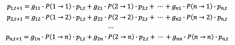
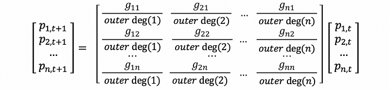
Write this difference equation as its matrix form, we can have,
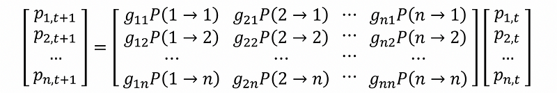
Because we have known that all the probability of i to j is exactly 1 divided by the outer degree of vertex i. Therefore,

Then, the equation system can be written as,
This is also,
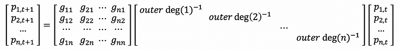
We can find out that the matrix consisted of gij is exactly the definition of the adjacency matrix of the directed graph G, therefore, if we define that,

Then,
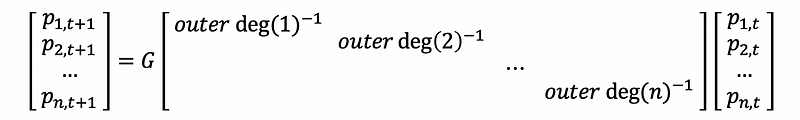
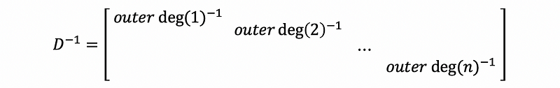
Suppose we define the diagonal matrix D as our degree matrix,

then based on the property of the diagonal matrix, we can have,
this is to say that, for the difference equation system, we can then have,

this is also,

(2) Proof of the Stochastic Matrix GD^(-1)
By definition of the inner product, we have,

Also, we have the expression of GD^(-1) as,
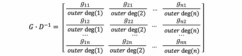
The sum of the entries in each of these columns should be,

Therefore, the matrix GD^(-1) is a stochastic matrix. Recall the property of the stochastic matrix, we can know that this matrix has a stable state p.
(3) Solve the Stable State of the Random Walk Problem
The stable state of the random walk problem gives us a final state of probabilities of each vertex. Suppose we have a stable state p and this stable state can have the property that,

then,

then,

then,

then,

(4) The Definition of the Laplacian Matrix
Suppose we have the adjacent matrix A of Graph G, and we also have the degree matrix noted as D. Then the Laplacian matrix is defined by,

If we have a non-directed graph (which means the outer degrees equal the inner degree) and there is no self-connected vertex (which means the main diagonal entries of A are 0). Then we can have,
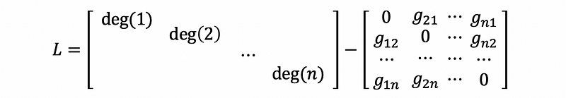
then,

So in general, for a non-directed graph, the entries in the Laplacian matrix are,

(5) Solve the Stable State of the Random Walk Problem (Continue)
Based on the previous discussion,
then, by Laplacian matrix,

this is also,

If we want to solve the stable state by this equation, this can be hard to calculate because this is going to take a long time for calculation. So have we got some easier methods?
(6) Recall: The Power Method
In the last section, for any given stochastic matrix M, if we power this matrix with N times and limit N to infinite, then it will give us the result of the stable state. A rigorous proof is as follows.
Proof:
Given a stochastic matrix M, and given ∀ vector x in ℝⁿ.
Suppose {v1, v2, …, vn} is a basis of ℝⁿ space and these vectors are also the eigenvectors of M, we can then write x as a linear combination of these vectors in the basis of ℝⁿ,

Then,

then,

then,

based on the property of the stochastic matrix M, we have,

when,

thus,

then,

if we let,

for any given x, we have p as our stable state,

Because the matrix multiplication is easier than solving equation systems, so we can compute the stable state of the random walking problem in this easier way.
3. Google’s Pagerank Algorithm
(1) Why Ranking Webpages Problem is a Random Walking Problem?
The concept of the internet is similar to a directed graph, with every IP address being treated as the nodes, and we can link different pages with hyperlinks.
The basic idea of PageRank is to rank the webpages based on the probability they pop up in the internet world. If a website has more sites directing to it, then it will have a higher probability to pop up on the internet. By this idea, we can calculate the stable state of the websites and rank them with these probabilities of the stable state.
Thus, based on the previous discussion, we have the stochastic matrix M of pagerank as,

where A is the adjacent matrix of the graph G and D is the degree matrix of the graph G. However, this matrix still have some issues and we have to solve all of them.
(2) Zero Outer Degree Issue
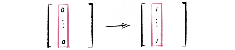
In the internet world, a node can have several edges pointing into it but no edges pointing out. Particularly in this example, the outer degree of this vertex equals zero and we can not construct a stochastic matrix M (because one column of M will be zeros).
One idea to solve this problem is to add a self-pointed edge that link back to this node. However, this idea is a misunderstanding because the random walking process will stuck in this loop forever.
Another idea is to jump randomly to any other nodes after this closed node. It is similar to add edges that point form the present node to all of the other nodes. Because this equals a random start from any of these node, so it actually didn’t change the relative rank of the stable state. Therefore, we can figure this problem out by exchanging the zeros in this column of A to a column of ones.
After this, we are glad to see that M is still a stochastic matrix.
Written by matrix, suppose we have a vector e which is,

also, we have a vector a where,

Therefore, we can construct a matrix by them and then add it to the adjacent matrix A,

Therefore, the adjusted stochastic matrix H is,

(3) Disconnected Graph Issue (Subnetwork)
The other issue is that we can have a disconnected graph that if we start from some part of the graph, we can never reach the other part of this graph.
One way to solve this problem is to add a teleportation matrix to the adjacent matrix so that on each of the vertex, we have a percentage to shift to another vertex. The teleportation matrix is a matrix with all entries equals one.

Because we still want M to be a stochastic matrix, so we have to normalize the result of M = H + T.
However, google chose another way to make this a stochastic matrix, they add a new parameter α in order to reduce the influence of the teleportation matrix. If we directly normalize this, we can have a high teleportation rate, although the result remains. In the area of computer science, it costs more for us to reach a stable state. Therefore, google adds a parameter α and then rewrite the stochastic matrix,

In practice, α is chosen between 0.8 ~ 0.85 by google. Although it will not influence the final rank by changing the parameter α, it reduces the cost of calculating when α is chosen between 0.8 ~ 0.85 (we are not going to prove this).
(4) Calculating the PageRank
We have already talked about the power method in the previous part, and then we utilize this method on the pagerank matrix M we have constructed, then,
Because p is not normalized in this case, so if we want to have the real probability, we can do normalization on p. But if our goal is to rank the webpages, then congratulations, you have already gotten the result! Now you’ve mastered the pagerank algorithm.