Linear Algebra 13 | Singular Value Decomposition, Pseudo Inverse, and Principal Component Analysis
Linear Algebra 13 | Singular Value Decomposition, Pseudo Inverse, and Principal Component Analysis

- Singular Value Decomposition
(1) The Problems of Eigendecomposition
Although the eigendecomposition can be useful sometimes, the strong condition of this makes it hard to utilize for any given matrix. The problems are as follows,
- S is usually not orthonormal (only for symmetric matrix)
- There can be not enough eigenvectors (when the algebraic multiplicity > the geometricity of an eigenvalue)
- The matrix to be decomposed must be a square matrix.
So we develop a new way to decomposition a matrix A, which perfectly solves all of these three problems.
(2) Recall: Eigendecomposition of the Symmetric Matrix
Suppose A is any m × n transformation matrix and A: ℝⁿ → ℝᵐ. If we then look at AᵀA, this is a symmetric matrix that has a basis of ℝⁿ consisting of eigenvectors and AᵀA is orthonormally diagonalizable.
So if we look at,

then the max value occurs in the direction of the eigenvector corresponding to the largest eigenvalue of AᵀA.
(3) The Definition of the Singular Value
We can take those eigenvectors of AᵀA to be an orthogonal basis. Suppose we assign that r = rank(A). Then we take the basis that {v1, v2, …, vr, vr+1, …, vn} corresponding to λ1 ≥ λ2 ≥ …≥ λr ≥ 0 = … = 0 (based on the fact of the semi-definite quadratic form).

For any λi > 0, we define that,

so that σ1 ≥ σ2 ≥ …≥ σr ≥ 0. These values σi are called the singular values.
(4) A Fact of the Singular Value
Because we have that,

then,

this is to say that,

thus,

(5) The Definition of the Singular Vector
Recall what we have learnt for the column space. Suppose we have a vector x and a transformation matrix A, then the vector Ax is a vector in the column space of A. Therefore, for the eigenvectors {v1, v2, …, vr}, we can conduct A transformation on them and throw them into the column space of A and finally, we will have a basis that {Av1, Av2, …, Avr}. Now we are going to claim that this is actually an orthogonal basis of the column space of A. How could it be possible? We have to prove our claim.
Proof:
We have already known that the transformation matrix A will throw v into the column space of A, then all vectors in the set {Av1, Av2, …, Avr} must be in the column space of A.
Also we have,

then for all i ≠ j, we can have,

then {Av1, Av2, …, Avr} is an orthogonal basis for the column space of A.
If we then normalize {Av1, Av2, …, Avr} as,

then the normalized vectors set {u1, u2, …, ur} is called the set of singular vectors of A.
(6) The Relationship Between the Singular Vector and the Singular Value
Based on the fact that,
then we can have,

This is the basic form for i of the singular value decomposition. Now let’s write the matrix form for this.
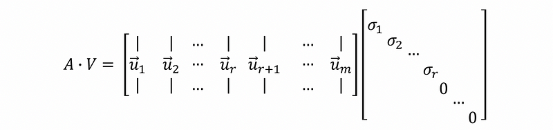
(7) Singular Value Decomposition
Suppose we define the n × n orthogonal matrix V as,

with the column vectors v1, v2, …, vr, vr+1, …, vn corresponding to the eigenvalues of AᵀA as λ1 ≥ λ2 ≥ …≥ λr ≥ 0 = … = 0.
Moreover, we define the m × m orthonormal matrix

then,

By,
when i = 1, 2 …, r and

otherwise.
Therefore, we can have,

This is also,

then,
then,

if we define that,

then we can write,

(8) The General Form of the Singular Value Decomposition
Because all the vectors {v1, v2, …, vr} is the eigenvectors of the symmetric matrix AᵀA. Therefore, it is clear that all these eigenvectors are orthogonal (we have used this conclusion before). Suppose these vectors {v1, v2, …, vr} are also normalized then we have an orthonormal basis vectors {v1, v2, …, vr}.
Therefore, the matrix V is an orthonormal matrix, and we can have that,

then, for
we can have that,

So in conclusion, the general form of singular value decomposition is,

where,
- U an m × m orthonormal matrix whose 1 ~ r columns are the basis of Col(A) and the r ~ n columns are a basis of N(Aᵀ).
- Σ is an m × n diagonal matrix with singular values
- V is an n × n orthonormal matrix whose columns are the eigenvectors of the symmetric matrix AᵀA.
2. Steps to Find a Singular Value Decomposition
Suppose we are given a matrix A, how we can find its singular value decomposition?
- Step #1
Compute AᵀA, find all the eigenvalues, and all the eigenvectors of AᵀA. Write down them in the order from the largest eigenvalue to 0, namely v1, v2, …, vr, vr+1, …, vn. Construct V by the results.
- Step #2
Compute u1, u2, …, ur, let them be the 1 ~ r columns of the matrix U and then find ur+1, … , un, to make {u1, u2, …, ur, ur+1, … , un} be a basis of ℝᵐ space. This step can be time-consuming and sometimes we have to use GS orthogonalization to get the full orthonormal basis of ℝᵐ space.
- Step #3
Compute the singular values and put them in the first 1~r rows of the diagonal matrix, set zeros to the other entries.
3. Pseudo Inverse
(1) The Definition of Pseudo Inverse
Suppose we define A-plus that satisfies,

then, A-plus is called the pseudo-inverse of A, where,

is a diagonal matrix with non-zero diagonal entries equal to,

(2) Two Facts of Σ-Plus
By definition, we can have the facts that,

and,

(3) The Results of Pseudo Inverse
We have,

then AA-plus is a projection matrix onto the column space of A.
We have,

then A-plusA is a projection matrix onto the row space of A.
4. Principal Component Analysis
(1) The Definition of Data Matrix
Suppose we have an n × p matrix X who has the form of,
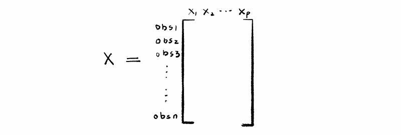
each column represents a different variable and each row is a single observation. Then we call this matrix X a data matrix.
(2) Singular Value Decomposition for Data Matrix
For a data matrix X, we can have its SVD as,

We can also write this as,

(3) PCA by a SVD Method
The goal of PCA is to find the principal component of a matrix.
Because we have ordered the singular value so that,

then the express in the front is more significant for the matrix X compared with later expressions (this is just a easy way to think about and definitely not a rigorous proof). Then we can reserve the first p dimension to get an approximation of matrix X.

By this mean, we can reduce a r-dimension matrix to p dimensions. This algorithm works well when we have small or medium datasets. For a large dataset, this is not the best way to conduct the PCA of a matrix.