Linear Algebra 16 | A Quick Review
Linear Algebra 16 | A Quick Review

- Vectors
(1) Definitions, stacking, slicing
- Defintion: a vector is an ordered list of numbers
- Stacked vector (concatenation): A stack vector of b, c, and d is a= [b, c, d]
- Size: the size of a vector is the number of entities in the vector
- Zeros: the zeros vector is the entities
- Ones: the ones vector is the entities
- Unit Vector: has one entry 1 and all others 0
- Sparsity: a vector is sparse if many of its entries are 0, nnz(x) is the number of entities that are non-zero
(2) Addition/subtraction, scalar multiplication
- commutative: a+b = b+a
- associative: (a+b)+c = a+(b+c)
- zero: a+0=0+a=a
- self substraction: a−a=0
- multiplication: βa = (βa1,…,βan)
- associative: (βγ)a = β(γa)
- left distributive: (β + γ)a = βa + γa
- right distributive: β(a + b) = βa + βb
(3) Inner product, norm, distance, RMS value
- inner product (or dot product) of n-vectors a and b is: aTb=a1b1 +a2b2 +···+anbn (a value)
- aTa=a1² +a2² +···+an² ≥0
- aTa=0 if and only if a=0
- commutative: aTb = bTa
- associative with scalar multiplication: (γa)T b = γ(aT b)
- distributive with vector addition: (a + b)Tc = aTc + bTc
- bombination conclusion: (a + b)T(c + d) = aTc + aTd + bTc + bTd
- Euclidean norm (norm): used to measure the size or magnitude of a vector

- Norm homogeneity: ∥βx∥ = |β|∥x∥
- Norm triangle inequality: ∥x + y∥ ≤ ∥x∥ + ∥y∥
- Norm nonnegativity:∥x∥ ≥ 0
- Norm definiteness: ∥x∥ = 0 only if x = 0
- RMS value: mean-square value of n-vector

- root-mean-square value (RMS value) is

Note that the RMS value is useful for comparing vectors of different dimensions
- Norm of block vectors

- Euclidean distance

- RMS deviation: rms(a -b)
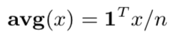
(4) Mean and standard deviation
- average definition vector form:
- de-meaned vector:

- standard deviation

- relationship between standard deviation, average, and rms

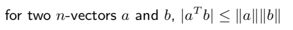
(5) Cauchy-Schwarz inequality, angle
- Cauchy-Schwarz inequality: can be used to prove the triangle inequality
- angle between two nonzero vectors a, b defined as

This is also,

- orthogonal angle: θ = π/2 = 90°, aTb=0
- aligned: θ = 0, aTb=∥a∥∥b∥
- anti-aligned: θ = π = 180°, aT b = −∥a∥∥b∥
- acute angle: θ ≤ π/2 = 90°, aTb≥0
- obtuse angle: θ ≥ π/2 = 90°, aTb≤0
(6) Correlation coefficient
- correlation coefficient (between a and b, with a ̃≠ 0,b ̃ ≠ 0)

Where,

This is also,

2. Linear Combinations
(1) Linear combination of vectors
For vectors a1,…,am and scalars β1,…,βm, then β1a1 +···+βmam is a linear combination of vectors.
(2) Linear dependence and independence
(3) Independence-dimension inequality
(4) Basis
(5) Orthonormal set of vectors
(6) Gram-Schmidt algorithm
3. Matrices
(1) Definitions, notation, block matrices, submatrices
- Definitions: a matrix is a rectangular array of numbers
- Size: (row dimension) × (column dimension)
- Entry: elements also called entries or coefficients
- Equality: two matrices are equal (denoted with “=”) if they are the same size and corresponding entries are equal
- Tall matrix: if m > n
- Wide matrix: if m<n
- Square matrix: if m=n
- Vector and matrix: we consider an n × 1 matrix to be an n-vector
- Number and matrix: we consider a 1×1 matrix to be a number
- Row vector: a 1 × n matrix is called a row vector
- block matrices: whose entries are matrices, such as

where B, C, D, and E are matrices (called submatrices or blocks of A)
- directed graph: a relation is a set of pairs of objects, labeled 1,…,n, such as


- n × n matrix A is adjacency matrix of directed graph:

- paths in directed graph: (A²)ij is number of paths of length 2 from j to i

- zero matrix: m × n zero matrix has all entries zero
- identity matrix: is square matrix with Iii = 1 and Iij = 0 for i ≠ j

- sparse matrix: a matrix is sparse if most (almost all) of its entries are zer
- diagonal matrix: square matrix with Aij = 0 when i ≠ j
- lower triangular matrix: Aij = 0 for i < j
- upper triangular matrix: Aij = 0 for i > j
- transpose matrix: the transpose of an m × n matrix A is denoted AT , and defined by

- Difference matrix: (n − 1) × n difference matrix is
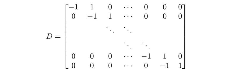
- Dirichlet energy: ∥Dx∥² is a measure of wiggliness for x a time series
(2) Addition/subtraction, scalar multiplication
- we can add or subtract matrices of the same size:

- scalar multiplication:

- many obvious properties, e.g.,

- matrix norm (Frobenius norm): for m×n matrix A, we define

- Norm properties #1:∥αA∥ = |α|∥A∥
- Norm properties #2:∥A + B∥ ≤ ∥A∥ + ∥B∥
- Norm properties #3:∥A∥ ≥ 0
- Norm properties #4:∥A∥=0 onlyif A=0
- matrix distance:∥A − B∥
(3) Matrix-vector multiplication, linear equations
- matrix-vector product: m × n matrix A, n-vector x, denoted y = Ax, with

- Row interpretation: y = Ax can be expressed as

- Column interpretation: y = Ax can be expressed as

(4) Matrix multiplication
- Multiplication: can multiply m×p matrix A and p×n matrix B to get C=AB

- out product: of m-vector a and n-vector b

- matrix multiplication property #1: (AB)C = A(BC)
- matrix multiplication property #2:A(B+C)=AB+AC
- matrix multiplication property #3:(AB)T =BTAT
- matrix multiplication property #4:AI = A and IA = A
- matrix multiplication property #5:AB ≠ BA in general
- Block matrix multiplication:

- Inner Product

- Gram matrix: must be invertible

- composition: define,

then,

- Second difference matrix:

- Matrix powers: for square matrix A, A² means AA, and same for higher powers
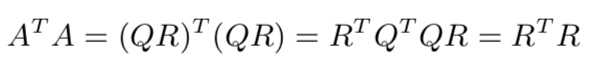
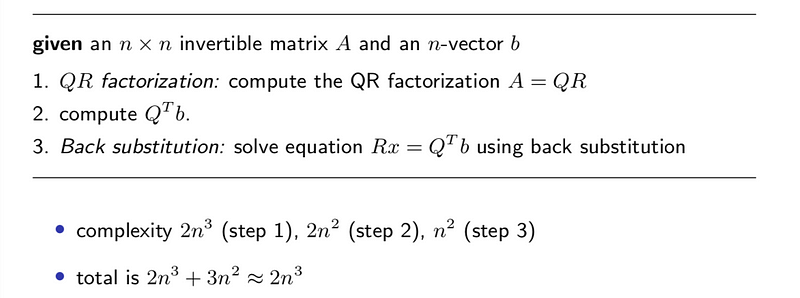
(5) QR factorization
- Gram-Schmidt:

where Rij = qiTaj for i < j and Rii = ∥q ̃i∥, so A=QR
- QR factorization of A: (1)QTQ=I; (2)R is upper triangular with positive diagonal entries
(6) Left and right inverses, pseudo-inverse
- Left inverse: a matrix X that satisfies XA = I is called a left inverse of A. If a left inverse exists we say that A is left-invertible
- Property #1: if A has a left inverse C then the columns of A are linearly independent

- Right Inverse: a matrix X that satisfies AX = I is a right inverse of A. If a right inverse exists we say that A is right-invertible.
- A is right-invertible if and only if AT is left-invertible:

Thus, a matrix is right-invertible if and only if its rows are linearly independent
- Pseudo-inverse of a tall matrix


- Pseudo-inverse of a wide matrix


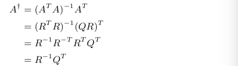
- Pseudo-inverse via QR factorization
pseudo-inverse gives us a method for solving over-determined and under-determined systems of linear equations. If the columns of A are linearly independent, and the over-determined equations Ax = b have a solution, then x = A†b is it. If the rows of A are linearly independent, the under-determined equations Ax = b have a solution for any vector b, and x = A†b is a solution.
(7) Inverse, solving linear equations
- invertible: if A has a left and a right inverse, they are unique and equal. A must be square

- suppose A is invertible, for any b, Ax = b has the unique solution

- inverse property #1

- inverse property #2

- inverse property #3

- inverse property #4

- Inverse via QR factorization

- The solution of the linear equations

4. Theory (linear algebra)
(1) Columns of A are independent ⇔ Gram matrix ATA is invertible
(2) A has a left inverse ⇔ columns of A are linearly independent
(3) (square) A is invertible ⇔ columns are independent, or rows are independent
5. Least-squares
(1) Basic least squares problem (Regression)
- residual: is r = Ax−b
- least-squares problem: choose x to minimize ∥Ax − b∥²
- objective function: ∥Ax − b∥²
- least-squares approximate: xˆ called least squares approximate solution of Ax = b
(2) Solution via pseudo-inverse, QR factorization
(3) Multi-objective least squares via weighted sum
(4) Equality-constrained least squares
(5) Solution via KKT system
6. Fitting models to data
(1) Least squares data fitting
(2) Regression model
- superposition property: f satisfies the superposition property if f(αx + βy) = αf(x) + βf(y), a function that satisfies superposition is called linear. The inner product function is linear

- Affine functions: a function that is linear plus a constant is called affine. general form is f(x)=aTx+b,with a an n-vector and b a scalar
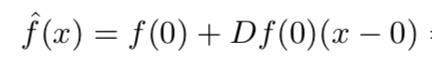
- Affine approximation: first-order Taylor approximation of f, near point z is,

This is also,

Where,

- Regression model is the affine function of x.

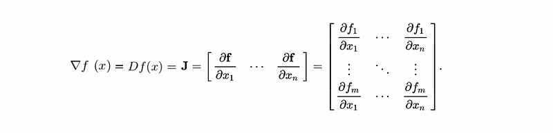
- Jacobian Matrix:
- First order Taylor approximation around z = 0
- associated predictions

- prediction error or residual (vector) is

(3) Validation on a test set
(4) Regularization
(5) Least squares classification
7. Computational complexity
(1) Floating-point operation (flop)
- flops: basic arithmetic operations (+, −, ∗, /, . . .) are called floating point operations or flops.
- running speed: current computers are around 1Gflop/sec
(2) Vector-vector operations (inner product, norm, ...)
- addition, substraction: n flops
- scalar multiplication: n flops
- inner product: 2n − 1 ≈ 2n flops
- norm: 2n − 1 ≈ 2n flops
(3) Matrix-vector multiplication, matrix-matrix multiplication
- matrix addition, scalar-matrix multiplication cost mn flops
- matrix-vector multiplication costs m(2n − 1) ≈ 2mn flops
- matrix-matrix multiplication costs mn2p = 2mnp flops
(4) QR factorization
- Total is 2n³ flops
(5) Inverse, solving linear equations
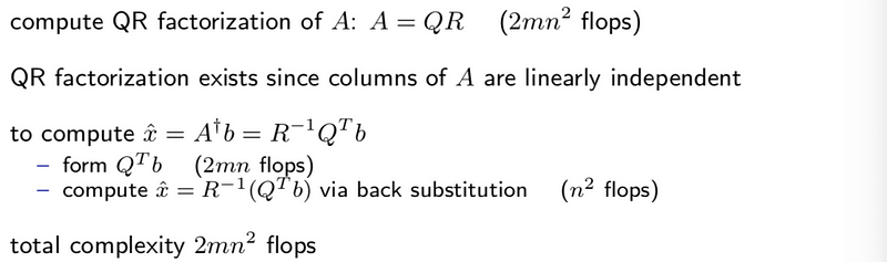
(6) Least-squares
(7) Linearly constrained least squares
(8) Backsubstitution
- back substitution total is 1+3+···+(2n−1) = n² flops