Linear Regression 1 | Basic Definitions, Simple Linear Regression, and Ordinary Least Square…

Linear Regression 1 | Basic Definitions, Simple Linear Regression, and Ordinary Least Square Estimation

1. Recall: Basic Definitions

(1) The Definition of Probability

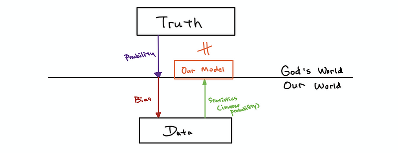
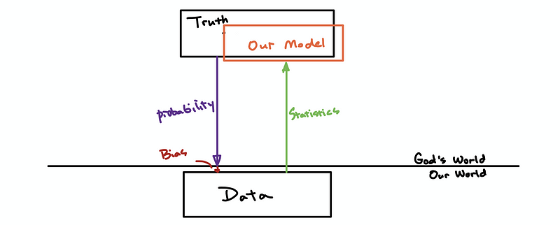
The probability is used when we have a well-designed model (truth) and we want to answer the questions like what kinds of data will this truth gives us.

(2) The Definition of Statistics

The statistics are used when we have a set of data and we want to discover the model or truth underlying the data. The statistics rely on the data and it is treated as the inverse of the probability.

(3) Probability vs. Statistics

You can find more information from this article:

So which one is more commonly used, statistics or probabilities? Well, it is hard to say, but we can confirm that most of the mathematics model we used today (i.e. there’s a 50% chance that it will be a rainy day tomorrow) is statistics and it is not the truth. The reason why we can make this assertion is that our models are based on the data but not the real mathematics models.

(4) The Definition of the Outcomes

In the probability theory, an outcome is a possible result of an experiment or trial. For example, if we flip a coin twice, the result of one flip is either head (H) or tail (T), so the outcomes can be one of the four consequences (H, H), (H, T), (T, H), or (T, T).

(5) The Definition of the Events

In the probability theory, an event is a set of outcomes. That means each event must contain at least one outcome, but they can contain as many outcomes as they like. For example, suppose we have several events A, B, and C,

• A = flip a coin twice, each outcome is either a head or a tail

⇒ A = {(H, H), (H, T), (T, H), (T, T)}

• B = flip a coin twice, with at least one tail

⇒ B = {(H, T), (T, H), (T, T)}

• C = flip a coin twice, with only tails

⇒ C= {(T, T)}

Usually, we use w to denote an event and we use Ω to denote the event that has all the outcomes of an experiment or a trial.

(6) The Definition of the Random Variables

The random variable is defined as a measurable function that takes on random values by any given events. The random variables are denoted as X(w) or X. For example, we define a random variable of X by the number of heads after flipping a coin twice, then X should be,

A loose definition of the random variables is that a random variable is a quantity that takes on random values related to our data. We are going to use this definition because this one is easier to understand.

(7) The Definition of the Bias

Suppose we conducted an experiment and then collected a set of data, what we want to figure out is that “why we have these data?”. The answer to this question is that it could be because of the truth of the underlying model (of the god’s world), or it can be because of the way we collected the data.

The truth of the underlying model, as we have said, can be stimulated by the statistics. However, because we can not estimate the impacts because of the experiment method, so we have to do our best to reduce the impact of the choice of the experimental methods.

This impact of the method is called the bias of the experiment.

We try to avoid the bias as much as possible so that we can have a better estimate of the truth,

(8) Two Schools of Statistics

Frequentist View - the parameters of probabilistic models are fixed, but we just don’t know them.

Bayesian View — the parameters of probabilistic models are not only unknown but also random.

(9) The Definition of the Probability Distributions

For a discrete random variable, the probability distribution p describes how likely each of those random values is. So suppose we have an observing value a and p(a) refers to the probability of observing a value a.

(10) The Definition of the Empirical Distributions

The empirical distribution of a dataset or usually called the distribution of the data is the relative frequency of each value in some observed dataset.

(11) The Definition of Expectation

The expectation of a random variable is the average value of this random variable. We often use the notation 𝔼 or μ to represent the expectation of a random variable.

(12) The Definition of Variance

The variance of a random variable is a measure of how spread out it is. We often use the notation Var or σ² to represent the expectation of a random variable.

(13) The Definition of a Sample Measure

The value we used to describe or summarize a sample is called a sample measure. It is denoted with a hat, for example,

(14) The Definition of Sample Mean

The mean value of the sample is the average value of a sample. The sample mean is a sample measure.

(15) The Definition of Sample Variance

The variance of a sample describes how spread out of data in a sample. The sample variance is a sample measure.

(16) The Definition of Unbiased Sample Measure

Mathematically, an unbiased sample measure should follow the feature that, on average, we do expect its value to be the real parameter of the truth.

(17) The Definition of the Standard Deviation

The standard deviation of a sample is the square root of its variance.

2. Simple Linear Regression and the Ordinary Least Square Solution

(1) The Definition of the Regression

The term of regression is invented by an English Victorian statistician named Francis Galton when he tried to describe the biological phenomenon that the heights of the descendants of tall ancestors tend to regress down towards a normal average.

(2) The Definition of Linear Regression

The linear regression is, literally, a regression that must have a linear form of a mathematical model. It is such an incredible and powerful tool for analyzing our daily data.

The term linear means that the parameters of this model should be linear instead of the variable itself. This can be hard to understand at the first glance. But we can think about the following examples,

These datasets can all be treated as a linear relationship. This is because we can produce them with a reproduce of xi, and the parameters will still be linear.

(3) The Definition of Simple Linear Regression

We are going to begin with the easiest model. Suppose we have got two variables and we would like to fit a line to our data. Define that x is our independent variable (aka. predictor variable) and y is our dependent variable (aka. response variable). For example, we have a dataset like

Then, we can fit a line with the form of,

where it is quite clear that β1-cap is the slope of the line and β0-cap is the intercept of the line. Note that we are using β0-cap and β1-cap and this is because we are not getting the real parameters, instead, what we are getting is the parameters based on our given data. So we can not directly write β0 and β1 in this case. Draw this line in the graph, which is,

But now, we have this line but we can not have the data. So this line seems meaningless. Suppose we are given every xi, we can still not exactly fit in the line to get all the yi. So what can we do now?

(4) The Definition of the Residual

Based on the line we have talked about, we are actually given is an estimator of yi (yi-cap) by given xi.

But, there is still a difference between yi-cap and the true value yi. And this difference changes when xi changes (so it is a random variable). We define the difference between the yi-cap and the true value yi as the residual of xi, which can be denoted as ei.

In the graph, we can randomly show an ei and an ej like,

Thus, in conclusion, the form of the simple linear regression for a given sample of two variables (or a dataset of two variables) is,

(5) The Definition of the Error Term

Previously what we are talking about is under the condition that we are given a sample or a dataset. So how about if we don’t have any samples or data and what is the truth behind two variables? Probably, suppose these two variables have a linear relationship similar to the above, we can then write a similar formula, which is,

In this formula, β0 and β1 are the true parameters and ϵi is called the error term. Here, the ϵi is also a random variable but it is very different from the residual ei. The residual can actually be seen as an estimator of the error term, but we can not call it in that way because ϵi is not a fixed value (instead, it is a random variable. We can only have an estimator of a fixed parameter).

What this formula means is that the god actually rolls the dice! We tried to grab a yi by a given xi, but the god will not give us the same value for the same xi, this is because that the god randomly chooses a random value and then add it to our result.

(6) Assumptions for the Error Term

So now we have known the definition of the error term and it should be a random variable, however, we can know nothing else from the previous discussion. This is absolutely not good for any further discussions. And there is a need we make an assumption of this error term in order to get more information.

First of all, we can have a strong assumption that gives all the information we need for this random variable. So,

• Assumption #1: the strong condition of Gaussian noise

But we can reduce the conditions or assumptions so as to make the conclusions more general, we have three loose assumptions here,

• Assumption #2: zero mean

• Assumption #3: population variance

• Assumption #4: no correlation between errors

For different assumptions, we can have different interesting conclusions. And we are now going to start with the assumption #1 and save the others for the later discussions.

(7) The Assumption for the Independent Variable

The independent variable is called so because we make an assumption of it. The assumption is that the independent variable has a fixed effect on the dependent variable. By this assumption, we don’t have to worry about how the distribution of the independent variable impacts the dependent variable.

(8) Solving For the Best Fit Line

Suppose we have a set of data (x1, y1) … (xn, yn), or a sample set or a set of observations, then it turns out that we can find as many lines we want to fit in the data. But there is only one line best fits all the data. This question is equivalent to solving the following optimization problem of the sum of the squares,

This is known as the least-squares linear regression problem (or the Ordinary Least Squares Regression Problem, or OLS). We can denote this as the function s, which is,

Thus,

(9) A Common Mistake

People usually mixed up the notations, sometimes I saw people sometimes write things like,

or,

These are completely meaningless because we can’t mix the notations up. Keep carefully in mind that ϵi is the error term for the truth and ei is the residual for the sample.

(10) Solving the OLS Estimator

By,

Now we would like to solve β0-cap and β1-cap. First of all, let’s use the partial derivation,

then,

then,

then,

then,

then,

Because,

then,

then,

This is the solution of the OLS estimator.

(10) The Second Solution of the OLS Estimator

By the result above, we can have,

then, we can have,

then,

then,

then,

then,

then,

Recall that the denominator is the sample variance of the independent variable and the molecular is the sample covariance of the independent variable and the dependent variable. Thus, suppose we have notation that,

then,

thus,

(11) The Third Solution of the OLS Estimator

Because we can know that the molecular is the sample covariance of the independent variable, then we can turn this sample covariance into a sample correlation.

The sample correlation coefficient is defined as,

where sx and sy are the sample standard deviation of variable x and y.

Then by,

we can have,

Because,

then,

then,

(12) The Fourth Solution of the OLS Estimator

Also, by

we can know that,

then,

then,

also, by previous discussion of the second solution,

Suppose we define that,

then,

(13) A Summary of the OLS Solution

Based on the discussions above, we can have that,

where,

and,

3. Evaluation the Ordinary Least Square Solution

(1) Gauss-Markov Theorem

The least-square estimators β0-cap and β1-cap are unbiased. This is to say that,

Proof:

We have defined ki satisfies

then,

moreover,

By the definition of the bias, we have,

because

then,

then,

Because we are under the assumption of a Gaussian distributed error term ϵi ~ N(0, σ²), then,

Also,

then,

For β0-cap, we have,

then,

then,

then,

Thus,

(2) Variance of the Estimator

Now we have known that the expectation of the estimators equals the true parameter under the Gaussian noise (error) assumption, so what are the variances of these two estimators?

Similarly, we have,

We have known that,

with β0, β1 fixed and given xi, the error term ϵi contributes all the variance of yi. Also, because ϵi ~ N(0, σ²), then,

then,

by the definition of ki,

then,

then,

thus,

For β0-cap, we have,

then,

then,

then,

then,

then,

with,

then,

then,

thus,

(3) Best Linear Unbiased Estimator

In fact, we give a very high evaluation of the OLS estimator under the assumption of the Gaussian noise, which is BLUE (full name: the best linear unbiased estimators). By the Gauss-Markov theorem, we can know that β0-cap and β1-cap are unbiased estimators.

Also, by the fourth solution of the OLS estimator, which is,

we can know that β1-cap is a linear estimator.

By what we have calculated in above,

this is to say that,

then, β0-cap is also a linear estimator.

We are going to leave an open question here. Why is OLS the best estimator? We are going to discuss it in the following sections.