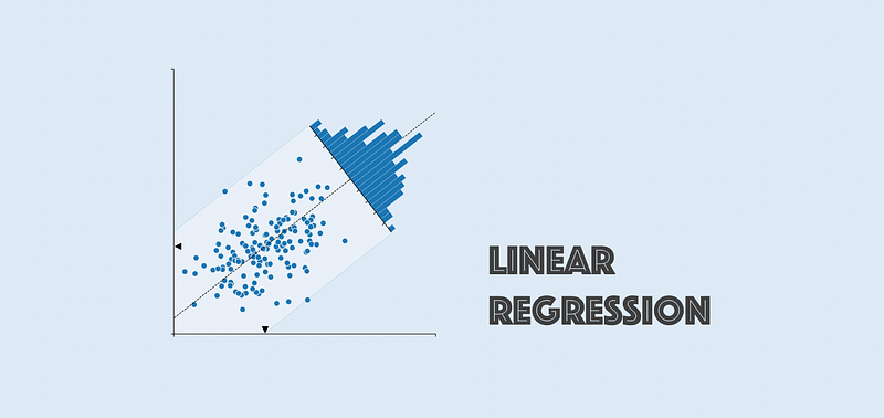
Linear Regression 2 | Properties of the Residuals and the ANOVA
Linear Regression 2 | Properties of the Residuals and the ANOVA
- Recall: Basic Definition
(1) The Definition of the Fitted Value
For a given xi, we can calculate a yi-cap through the fitted line of the linear regression, then this yi-cap is the so-called fitted value given xi.

(2) The Definition of the Residuals
As we have defined, residual is the difference between the yi-cap and the true value yi as the residual of xi, which can be denoted as ei.

Thus, by the mathematical model of the linear regression, we can have,

(3) The Definition of Prediction
At a particular x*, we can use the fitted line to calculate the fitted value y-cap(x*) and we can do this even if x* is NOT in our original dataset. If this x* is not in our original dataset, then this y-cap(x*) is called a predictor.


(4) A Critical Conclusion by Mean
By definition of the sample mean of xi, we can derive that,

Also, because x-bar is a constant,

thus,

then, the first central moment of xi must equal to zero,

and the second central moment can be as follows,

Also, with,

then,

2. Properties of the Residual
- Property #1: Zero Sum

This is not an assumption since we are already under the assumption of a Gaussian distributed error.
Proof:

then,

then, by solution of the OLS,

- Property #2: Zero Expectation

Proof:
By the zero-sum property,

- Property #3: Zero Covariance for One Term
In order to get this assumption, we have to make a crucial assumption, we want it to be the case that knowing something about x does not give us any information about e, so that they are completely unrelated. That is to say that,

Based on this assumption, we can know that the covariance of the residual e and any term in the regression model is zero, that is,

Proof Method #1: with the crucial assumption
First of all, by the law of iterated expectations,

then by conditional rule,

then because we are under the crucial assumption that,
This is to say that,

Then we can know that, because,

then,

By the definition of the covariance,

by property #2,
then,

thus,

Proof Method #2: without crucial assumption
Let’s see, what if we loose the previous assumption. This is quite interesting because we are going to use this for further discussions. We have already known than
Suppose we don’t have the property #2 and we don’t have the assumption that,
What we only have is that,

can we still have this conclusion that the covariance of the residual e and any term in the regression model is zero? The answer is yes, and here’s our proof:
First of all, by the law of iterated expectations,
then by conditional rule,
then because we are under the assumption that,
then,

thus,

By the definition of the covariance,
then,

Thus, we can find out that the 0 covariance property holds if we are only given the assumption that,

- Property #4: Zero Covariance for All Terms

Proof:
By the fitting line,

then,

then,

then,

then,

by the law of iterated expectations,
then by conditional rule,
then because we are under the assumption that,
then,
thus,
then,

thus,

Also, to have this conclusion, what we only need to assume is,
3. Parameter (Estimator) Distribution and Estimator Testing
(1) Recall: The Variance of the Estimator
Based on our discussion in the last section, we can have that,

and,

However, notice that we have a problem that we don’t know anything about the σ² in practice, because we don’t have the statistics about the truth by any given dataset. Thus, in fact, these formulas are only valid in the theory.
(2) The Definition of the Sum of Squared Errors (aka. SSE)
We have already the residuals in the discussions above, and now, we would like to given the definition of the sum of squared errors. Actually, it is called the sum of squared errors but it is actually not a sum of square errors. It is in fact defined by the sum of square residuals and this can be quite tricky. This is to say that, we define

Based on the OLS, we can know that the estimators are BLUE if SSE is minimized. By our model and the Gaussian assumption, we can know that,

Also,

then,

(3) Recall: Chi-Square Distribution
If X1, …, Xn are independently identical distributed (aka, i.i.d) normal random variables with mean μ and variance σ², then,

(4) The Definition of Degree of Freedom to the Residuals
In linear regression, the definition of the degree of freedom to the residuals is the number of the instance in the sample minus the number of the parameters in our model (of course, including the intercept). This is to say that,

Particularly, in the model of SLR, because we have two parameters (a slope and an intercept), then we can conclude that the degree of freedom for SLR is,

(5) The Definition of the Mean of Squared Errors (aka. MSE)
Because y1, …, yn are independently identically distributed normal random variables with the mean (β0+β1x1) and the variance σ², then by the definition of the Chi-Square Distribution, we can conclude that,

This is not a formal rigorous proof, and I will add a more rigorous if time permits in the future.
Buy this formula, we can know by the property of the χ² distribution,

Because n-2 and σ² are all constant, then,

Suppose we define the mean of squared errors (MSE) as,

Then we can have that,

This means that MSE is an unbiased estimator of the population variance. Thus, we can use this to replace σ² for estimators if we are given only a dataset.
(6) Estimator Distribution with known σ²
By our previous discussions, when we have a known σ², then,

also,

(7) Estimator Distribution with unknown σ²
Suppose we don’t have a given σ², then, the distribution of β1-cap is a student’s T distribution.

This is also to say that,

and this is also,

(8) Application of the Estimator Distribution: Significance Testing
Because we have known the distribution of the estimator, then we are able to test whether an estimator is significant by hypothesis testing. We can define the null hypothesis Ho: β1 = 0, and the alternative hypothesis H1: β1 ≠ 0. By this method, we can know that, if we can reject Ho, we can know that H1 is significant on the given significant level. Thus, we can have the T statistics equals,

If,

or,

then, we are able to reject Ho. And this is equivalent to say that the independent variable x is significant to the dependent variable y.
3. ANOVA
(1) The Introduction of ANOVA
The whole name of ANOVA is called the analysis of variance, and it is a way for us to test the significance of more than one parameter. It is more commonly used in MLR (multiple linear regression) it saves time to test that if there’s any parameter that is not significant. ANOVA also tests the interval parameter in SLR.
For SLR, we can have the following ANOVA table,
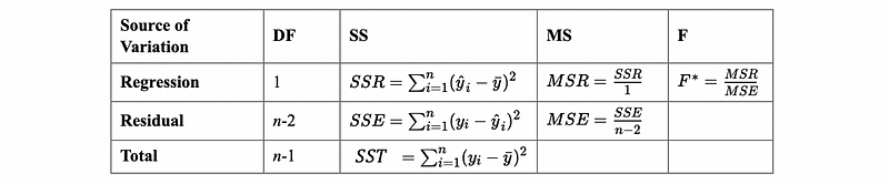
(2) The Definition of the Total Sum of Squares
The total sum of squares is the variance given the total dataset. Thus, by the definition of the sample distribution, we can then have,

(3) The Definition of the Regression Sum of Squares
The total sum of squares is the variance given by values generated by the fitted line. It is actually the natural variance of variance that we can get if x is strictly and linearly related to y. So the source of this variance is from the regression itself.

(4) Total Sum of Squares Explanation
Based on the definitions above, we can have the theorem that,

This is also to say that,


Proof:

then,

because

then,

then,

then, by property #1 and property #3 of the residual,

thus,

thus,

(5) ANOVA F Testing for SLR
Suppose we have an SLR model and we would like to test Ho: β1 = 0. By ANOVA, we can then conduct F testing. This is called an ANOVA F testing.
The reason why we can use F testing is that, when β1 = 0, we are able to draw the conclusion that,

this means that the residuals contribute all the variance and the independent variable can not explain anything of the variance.
However, when β1 ≠ 0, we are able to draw the conclusion that,

Thus, we are expecting,

for a given sample, both MSR and MSE are unbiased, thus,

Because MSR and MSE are two variances with degrees of freedom 1 and n-2 respectively, thus, based on the definition of F distribution, we can know that the ratio of them follows,

Thus, we reject Ho if,

or,

and then we can confirm that the parameter β1 is significant.
(6) The Definition of the Goodness of Fit (aka. R-Square or R²)
If we want to measure how much the variance is explained by our model, then we can define this with a ratio of SSR over SST. This is to say that,

This is called the goodness of fit or R-Square.
(7) Second Form of Goodness of Fit
The goodness of fit can also be the square of the sample correlation between x and y,

We are not going to prove this here, but we can have a quick reference from the following link.
The conclusion of this is that R² is a constant from 0 to 1 and we are able to say that, when R² is closer to 1, then this indicates a better fit of the model.