Linear Regression 3 | Distribution of the SLR Estimators, SLR Measures, and Python Implementation…
Linear Regression 3 | Distribution of the SLR Estimators, SLR Measures, and Python Implementation of SLR
- Recall: Distribution of the Estimators
(1) The Definition of the Estimators
The estimators are the specific values we calculated by given our specific dataset that is used for estimating the true value of the truth. The most valuable estimator is the unbiased estimator because the expectations of the unbiased estimators equal the true values (with some mathematical proof) of the truth. Thus, for expressions including the true values, we can then replace them with the unbiased estimator because the expectation of this won’t make any change, although we have added the costs of the variances.
What’s more, these variances are going to tell us new stories of the true values and we can use the variance and the expectation of the estimator to tell what might be the true value (actually a range under a certain confidence level). And because we don’t want the true value to be some specific values like 0, so must be able to confirm that 0 is not in the range (confidence interval) of the true value.
For SLR, suppose we are under the estimation of Gaussian errors, so what we have as our estimators are,
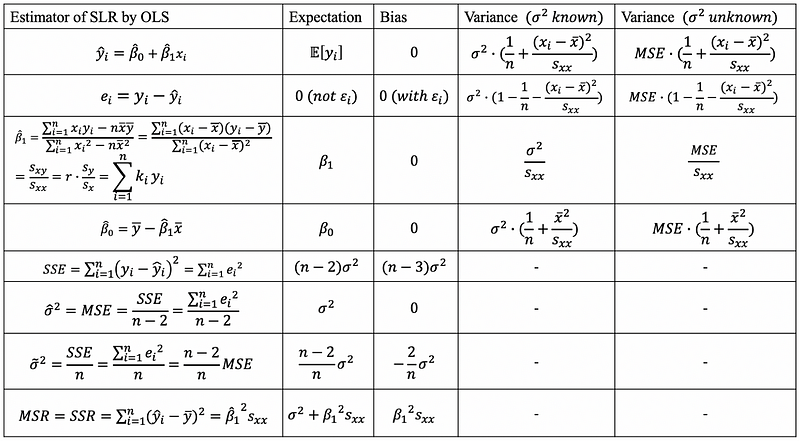
Let’s now do all the proofs again to make things clear and easy for us to understand.
(2) Proof of OLS estimator β0-hat and β1-hat
By,

Now we would like to solve β0-cap and β1-cap. First of all, let’s use the partial derivation,

then,

then,

then,

then,

then,

Because

then,

then,

This is the solution of the OLS estimator.
Also, we can have,

then,

then,

then,

then,

then,

(2) Expectation of OLS estimator β0-hat and β1-hat
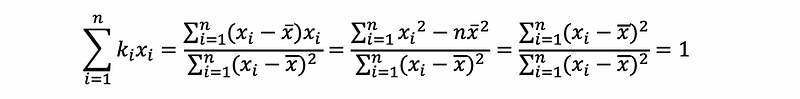
We have defined ki satisfies

then,

moreover,

By the definition of the bias, we have,

because

then,

then,

Because we are under the assumption of a Gaussian distributed error term ϵi ~ N(0, σ²), then,

Also,

then,

For β0-cap, we have,

then,

then,

then,

Thus,

(3) Variance of OLS estimator β0-hat and β1-hat
We have defined ki satisfies

then,

moreover,
we also have,

We have known that,

with β0, β1 fixed and given xi, the error term ϵi contributes all the variance of yi. Also, because ϵi ~ N(0, σ²), then,

then,

by the definition of ki,

then,

then,

thus,

For β0-cap, we have,

then,

then,

then,

then,

then,

with,

then,

then,

thus,

(4) Expectation and Variance of the Fitted Value yi-cap
For yi-cap,

because xi is fixed,

Based on the fact that,
then,

thus,

Also, we can have that,

then,

then, because xi is fixed,

then,

By OLS,

then,

then,

then,

then,

then,

(5) Expectation and Variance of the Residual
For the residual ei,

because

then,

then,

for variance,

then,

Moreover,

then,

Given the assumption that,

By the fitting line,

then,

then,

then,

then,

by the law of iterated expectations,

then by conditional rule,

then because we are under the assumption that,

then,

thus,

then,

thus,

then,

then,

then,

By the fact that,

then,

(6) Expectation of MSR
By definition,

because by OLS,

then,

thus,

So,

then,

also by definition of the variance,

then,

then,

2. Measure of the SLR
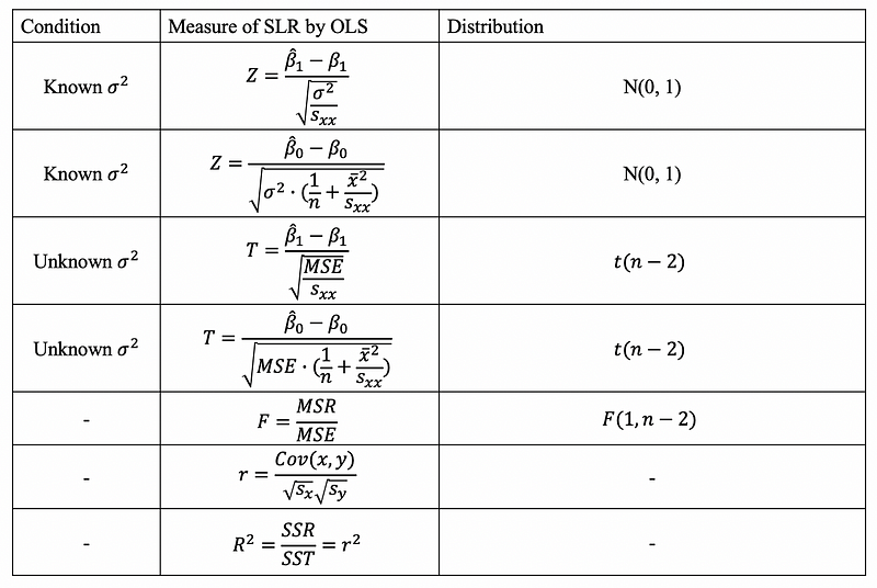
In fact, there are also many measures that we have to pay attention to for the simple linear regression. We can use these measures to tell whether or not this SLR is a good statistics model or not.
For SLR, suppose we are under the estimation of Gaussian errors, so what we have as our measures are,
3. Python Implementation of SLR
(1) Linear Regression with Sklearn
- generate the model
from sklearn import linear_model
reg = linear_model.LinearRegression()
reg.fit(x, y)
- get the estimators
coef = reg.coef_
intercept = reg.intercept_
- predict a value
x0 = [12]
y0 = reg.predict([x0])
- predict values
xs = [12, 13, 14]
ys = reg.predict([xs])
(2) Linear Regression with statsmodels.api (aka. sm)
- generate the model
import statsmodels.api as sm
x = sm.add_constant(predictor)
model = sm.OLS(y, x).fit()
- get the estimators
model.summary()
- predict a value
x0 = [[1,12]]
y0 = model.predict(x0)
- predict values
xs = [[1,12], [1,13], [1,14]]
ys = model.predict(xs)
(3) Linear Regression with statsmodels.formula.api.ols (aka. smf)
- generate the model
import statsmodels.formula.api as smf
model = smf.ols('y ~ x', df).fit()
- get the estimators
model.summary()
- predict a value with CI
x0 = [12]
prediction=model.get_prediction(exog=dict(x=x0))
prediction.summary_frame(alpha=0.05)
- predict values with CI
xs = [12, 13, 14]
prediction=model.get_prediction(exog=dict(x=xs))
prediction.summary_frame(alpha=0.05)
(4) Analysis of Variance (ANOVA) With sm And smf
- import packages
import statsmodels.api as sm
import statsmodels.formula.api as smf
- generate the model with smf
model = smf.ols('y ~ x', df).fit()- generate the ANOVA table with sm
sm.stats.anova_lm(model, typ=1)