Linear Regression 7 | MLR Inference, Adjusted R-Square for MLR, Dummy Encoding and One-Hot Encoding
Linear Regression 7 | MLR Inference, Adjusted R-Square for MLR, Dummy Encoding and One-Hot Encoding
- MLR Inference
(1) F Statistics
As what we have discussed, similarly, the F statistics for MLR is defined by,

Suppose we have a more general case that is for some of the terms in a linear model, we want to test whether there’s at least one parameter not equal to 0. Denote the full model as ‘F’ and the partial model as ‘R’, then we have the statistical inference as,

Note that this is not strictly correct because the H1 hypothesis is no need to be F, it can actually be something between R and F (not including R).
And the F statistics can be written in a more general way as,

It is also clear to see that when we want to test all the terms except for the error term in an MLR model, then,

this is also,

(2) Student’s T Statistics
Based on our previous discussions,

Similarly to SLR, the t-test for the j-th individual coefficient is,

then, when σ² is known,

when σ² is unknown,

where,

(3) R²
Similarly to SLR, the definition of R² is,

(4) A Misunderstanding for R²: The Underfitting Problem
Sometimes we generate a model and find out all the parameters are significant at the 95% level. However, it is the low R² makes us nervous about our final results. For example, we may have an R² = 2% which indicates that the model is really bad and there are also many other explanatory variables not being included. This is commonly called an underfitted model or an underfitting problem.
But to have an underfitted model doesn’t mean that our model is not significant. Although it can be really bad for prediction, it can actually include some critically significant variables in the model. Many people misunderstand the meaning of the R² and they change the explanatory variables after they have a low R². Well, to some extent, this can work, but a wiser idea is to add more significant explanatory variables into the model until you a higher R². But if you don’t want to make predictions or if the full model is not so important for you, it’s okay if you report a low R².
But it can also be a really bad idea if we have too many explanatory variables in the model and get a really big R². This is the overfitting problem that we are going to introduce.
(5) The Overfitting Problems for R²
Let’s think about a problem, if I keep adding significant explanatory variables into the linear model, what can we finally have? Actually, we are going to have a model with a higher and higher R² and this is nothing strange by the definition of the SSR (we are not going to prove this here but you can have a try).
With more explanatory variables (whether or not they are significant or not) being added, we can find that is harder to tell the relationship between these newly added variables and the dependent variable. And it can also appear that even though our model more and more fits our model, it will become really bad for prediction because the model is overly explained by the redundant variables and it randomly tells the story about the noise in the data set. That’s why this model is bad if we have an overfitting problem.

However, can R² tells us that there’s an overfitting problem in the model? No, because the R² will be larger and it implies that the dataset is well explained by the model. So our question is that, is R² a good measure for an MLR model? Probably NOT when there’s an overfitting problem! Because we can actually know nothing about whether it is overfitting or not if we use only R² as our measure. That’s why we have to find a new measure for our model.
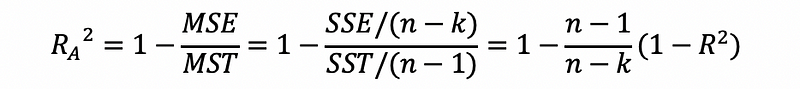
(5) The Definition of the Adjusted R²
The adjusted R² is an alternative to R² and it tells us whether or not this is an existing overfitting problem in the model. How come? The problem when we are adding new variables to the model is that we actually not only add the variance of the regression but also we reduce the degree of freedom. There are to ways that we can have a higher R² based on its following definition,

- get a higher MSR => what we want
- get a higher k => to add more explanatory variables and the model can become overfitting
Suppose we want to make a new measure that will not count the degree of freedom so that a higher k won’t affect our measure to some extent. There can be two ways to construct this measure. Then the definition of the adjusted R² is defined by,
(6) Increasing Adjusted R² Or Decreasing Adjusted R²
There are two cases when the adjusted R² will be increasing (or decreasing),
First, adding a regressor will increase (decrease) adjusted R² depending on whether the absolute value of the t-statistic associated with that regressor is greater (less) than one in value. Adjusted R² is unchanged if that absolute t-statistic is exactly equal to one. If you drop a regressor from the model, the converse of the above result applies.
Second, adding a group of regressors to the model will increase (decrease) adjusted R² depending on whether the F-statistic for testing that their coefficients are all zero is greater (less) than one in value. Adjusted R² is unchanged if that F-statistic is exactly equal to one. If you drop a group of regressors from the model, the converse of the above result applies.
There are religious proofs for these two cases and you can refer to click me and click me for more information.
(7) Negative Adjusted R²
Surprisingly, the adjusted R² can be negative. This is because it is actually not a must for our measure to be positive if the negative values are not too large and we can also have 1 as our upper bound of the method.
2. Dummy Variables in MLR
(1) The Definition of the Category Variable
The category variables are variables that take a limited and fixed number of possible non-ordered values. For example, gender is a kind of category variable that takes the non-ordered value of female or male.
(2) The Definition of the Dummy Variable
The dummy variable is a kind of variable that only takes only the value 1 and 0. And the meaning of 0 is that we haven’t got this effect and 1 is that we have this effect. There’s no order between 0 and 1.
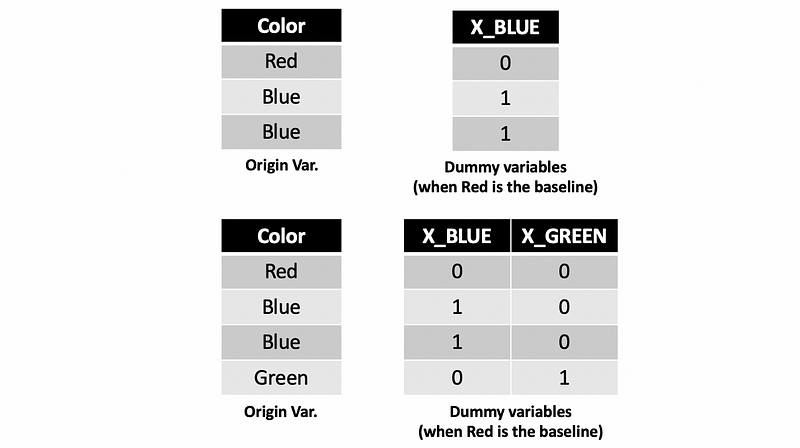
(3) Dummy Encoding
Dummy encoding means to code a category variable with k different values to k-1 dummy variables. We can not set the values of 0, 1, 2, … because this will imply the order of the category value.

(4) One-Hot Encoding
Dummy encoding means to code a category variable with k different values to k dummy variables. We can not set the values of 0, 1, 2, … because this will imply the order of the category value.
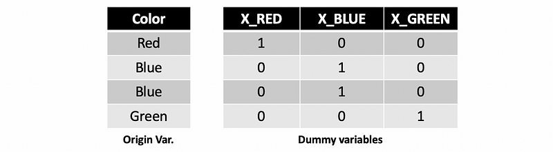
Note we are not going to focus on the one-hot encoding in this section.
(4) The Definition of the Baseline
The baseline value is the value that after a dummy encoding process, the value of the total when all dummy variables equal to zero. Actually, the impact of the baseline value has been added to the intercept parameter. We define the baseline because, by this means, we can reduce a dummy variable.
(5) Interpretation of the Parameter of the Dummy Variable
Because the dummy variable only has two values 1 and 0,
- For dummy encoding, the coefficient of a dummy variable in a linear model measures the change (or difference) caused in y when the observation is in the dummy level compared to the baseline level.
- For one-hot encoding, the coefficient of a dummy variable in a linear model measures the impact of a dummy variable on the dependent variable.
For python, by default, we are going to model with the dummy encoding method.
(5) Student’s T-Test for Dummy Variable
The student’s t-test for dummy encoding examines the significant difference between the other values and the baseline value (reference level). While, for one-hot encoding, it examines the impact of each value on the dependent value.
(6) ANOVA with Dummy Variable
Suppose we three values (i.e. blue, red, green) of a category variable (i.e. color), and by python, this variable will automatically be dummy encoded to 2 dummy variables and the ANOVA will test on the model after the dummy encoding.
For type I ANOVA, the F statistics will tell the sequence result based on the order of the independent variables being added to the model. If F statistics for type I ANOVA is significant, that means there’s at least one of the parameters for these 2 dummy variables is not 0 given the reduced model.
For type II ANOVA, the F statistics will tell the partical result. If F statistics for type I ANOVA is significant, that means there’s at least one of the parameters for these 2 dummy variables is not 0 given the reduced model.
Note that the degree of freedom of the category variable will be the number of the values of this category variable k minus 1 (or k-1).
To force a numeric variable as a category variable in python, we can use,
model = smf.ols('y~C(x)', data=df).fit()(7) Remaining Problems for Dummy and One-Hot Encoding
For dummy encoding of a categorical variable, we have to add k-1 dummy variables based on the number of different categories k. For one-hot encoding, we have to add k dummy variables. Then there will be two issues because of this,
- Multicollinearity (which we are going to introduce later)
- Not enough data (In linear regression, we want the #of parameters < the # of the observations, and it will be nice if we have # observations surpass 10~20). (which is the field of power analysis)