Linear Regression 9 | Model Diagnosis Process for MLR - Part 1

Linear Regression 9 | Model Diagnosis Process for MLR - Part 1

1. Model Diagnosis Process for MLR

(0) Goal of Modeling

• make prediction
• capture the significant predictors
• explain the changes in the dependent variable

(1) Step 1. Check Multicollinearity

• Reason: two predictors are correlated or highly correlated.
• Worst result: XtX is non-invertible (singular) and we can not calculate its inverse matrix. Thus, the OLSE can’t be achieved.
• Worse result: XtX is close to non-invertible, and we are going to have a matrix of inverse XtX matrix with huge values.
• Symptom

a. OLSE changes hugely when adding or dropping independent variables to or from the model, this implies that the newly added or dropped variable has a multicollinearity problem with the other variables in the model (sometimes even changes the sign);

b. It can be hard to reject the null hypothesis and there are several variables in the model that are not significant in the t-test. This is because the variance of the OLSE σ²inverse(XtX) can be huge, which makes the standard error for each OLSE large, and it contributes to a small t statistics in our model.

c. The sum of squares change a lot in the type 1 ANOVA test.

• Detection

a. Pairwise Correlation Plot: Heatmap correlation plot between predictors

b. Variance Inflation Factor (VIF): measures how much the variance is inflated in the coefficient estimates caused by an independent variable xj

Where Rj² is from the model xj ~ x1 + x2 +… + x(j-1) + x(j+1) +… + xk.

This measures how much variance is inflated by xj. Empirically, if VIF is between 1~10, then we think this inflation is okay are we are not going to think that there’s a serious multicollinearity problem in the model. However, if VIF is larger than 10, we can draw the conclusion that xj is causing a multicollinearity problem.

This also means that it’s not a good idea if you have an R² of more than 0.9 and you choose to add more explanatory variables into the model.

• Solution

a. Fast Solution: Drop some highly correlated variables.

b. Seldom used: Use a linear combination of highly correlated variables (especially they are on the same scale).

c. Regularization: the simple idea is to standardize the data so that the variance of each OLSE won’t impact too much of the general result

d. PCA: principal component analysis is actually a good way to reduce the multicollinearity problem, but it can make it hard for us to interpret the data

e. Partial Least-Squared Regression: just also another method, and we don’t have to understand this.

• Note

If dropping 1 or 2 variables, there’s still a multicollinearity problem, then just stop the dropping and leave the model there.

(2) Step 2. Fit the Initial Model

This step is to fit the data in our model, as we have done before. The first model that we generate is called the initial model.

(3) Step 3. Check Influential Points

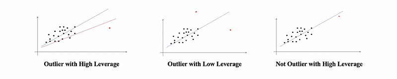
• Outlier: An observation has a response value yi that is very far from yi-hat
• High Leverage Point: An observation that has an unusual combination of predictor values that could influence yi-hat
• Inferential Points Problem: An observation that is both an outlier and has high leverage that impacted the fitted model significantly, is called the influential point problem.

• Effects of Inferential Points Problem

The influential points significantly affect the model estimation, because with or without these influential observations will lead to significantly different models.

• Detection

a. Detect Outliers

(i) with Semi-Studentized Residual (this is called semi because the estimated variance of ei is not MSE).

The rule of thumb is when |ei*|>3, then the point i is probably an outlier.

(ii) With Internal (read) Studentized Residual

Recall what we have studied for the residuals of MLR, the difference between the observed values and the fitted values is called the residual, and

Then the variance of the residual is

Based on the assumption of normality,

then,

then,

when σ² is unknown, then we can use MSE to estimate it, then,

Then the internal studentized residual is,

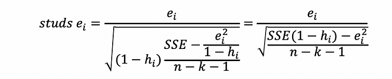
(iii) With External Studentized Residual (also detect the influence)

The external studentized residual can decide both the outliers and the influence of a point, which is defined as,

Proof:

where MSE(i) is defined as the MSE of the data removing point i,

then,

thus,

Proved.

Then to use this result to show whether a point is an influential outlier or not, this statistic of the external studentized residual follows,

So when,

then we can detect that the i-th observation is an influential outlier with a high influence.

b. Detect High Leverage with the Hat Matrix

Suppose we are given the hat matrix of an MLR, then the i-th row and i-th column entity of the hat matrix is defined as the leverage of the i-th observation.

The properties of the leverages are,

i. Ranging between 0 and 1

ii. Trace of the hat matrix

Proof:

iii. Average Leverage

iv. Rule of Thumb

An observation with,

can be considered as the high leverage points.

c. Detect High Leveraged Outliers (Influential) with Cook’s Distance

We don’t have to fully understand this, instead, we have to remember the conclusion of the Cook’s Distance and how it can be used to detect the influential outliers.

The Cook’s distance for the i-th observation is defined as,

where,

yj is the jth fitted response value and yj(i) is the jth fitted response value, where the fit does not include observation i.

Another expression (with the same value) of Cook’s distance is,

A more detailed explanation of the Cook’s distance can be found here,

The rule of thumbs with the Cook’s distance is that the observation is an influential outlier when Di > 4/n, where n is the number of total observations.

(4) Step 4. Check Heteroscedasticity

• Reason: We have to maintain the model assumption of the constant variance σ² for all error terms.
• Heteroscedasticity: occurs when this assumption is violated, which means the variance of errors are non-constant. More commonly, it refers to the spread of the residual changes
• Symptom:

a. The OLS estimate β is still linear and unbiased, but it is not the best estimate any more. We can not say β has the smallest variance among all unbiased linear estimators. There’s another estimator with a smaller variance.

b. The standard error of βk-hat for all OLS output are incorrect estimate of the standard deviation of βk-hat. It will result in a misleading t-test and a misleading confidence interval.

c. Predictions of y are still unbiased, but the prediction intervales are incorrect.

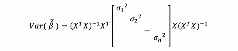
d. Variance-Covariance Matrix of the OLS Estimators

Recall the variance-covariance matrix of OLSE for MLR,

When, heteroscedasticity exists, the real variance of β-hat is,

then, because the constant variance assumption no longer holds, then,

thus,

so the estimate of,

Then, if we keep applying the OLS method,

i. Not the Best Estimator

ii. Biased Estimator

is now a biased estimator and the standard error of the β-hat is incorrect.

iii. The Predictions and the Confidence Intervals will be Incorrect

Recall what we have learned for the variance of the fitted value,

When there’s no heteroscedasticity,

Then the confidence interval for the observation i is,

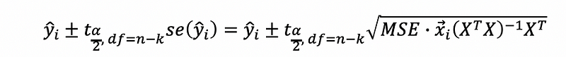
where, xi is the transpose of the i-th row in the matrix X.

also, the prediction interval for the observation i is,

However, when heteroscedasticity exists,

But, because

So,

Therefore, the prediction / confidence interval calculate by OLS estimator would be incorrect.

• Detection

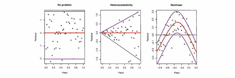
a. Residual vs. Fitted Value Plot

The model will be observed obvious change of the bandwidth in the plot with the given data if there’s a heteroscedasticity problem.

b. Breusch-Pagan Test (BP Test)

The basic idea of this test is that the variance of the errors should not change given difference predictor values. If the assumption of constant variance is violated, then the variance would be changed with predictor values.

i. Process of the Breusch-Pagan Test

Step 1. Fit the MLR model.

Step 2. Obtain the residual.

Step 3. Build an auxiliary regression model (this is called auxiliary because it does not estimate the model of primary interest)

And obtain R² value of this model.

Step 4. Hypothesis Testing

The testing statistic is,

The testing result is,

when fail to reject H0,

then we can conclude that there’s no significant heteroscedasticity problem at the 100(1-α)% confidence level.

when reject H0,

then we can conclude that there’s a significant heteroscedasticity problem at the 100(1-α)% confidence level.

c. White Test (A more advanced BP test)

We will not cover this now, maybe later.

• Solution

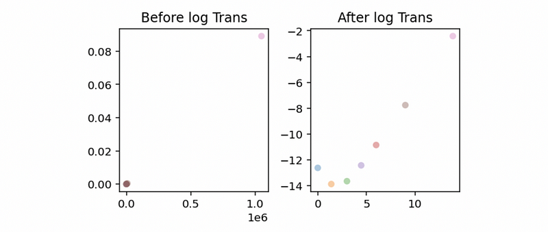
a. Log-Transformation on y: The natural log with e as its base is the most common transformation in MLR. This will be working because the small values that are close together are spread further out and the large values that are spread out are brought close to each other. See an example of this,

Now, let’s download this dataset. We’ll use Accident as the dependent variable and Population for the independent variable. Then, the following program is to draw a residual vs. fitted value plot,

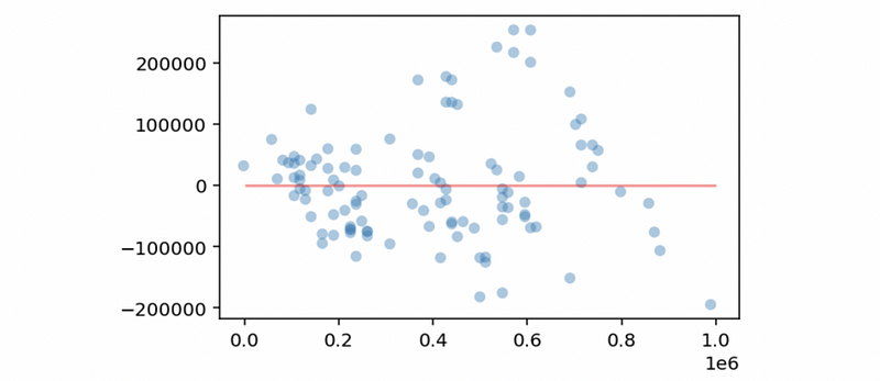
We can detect a heteroscedasticity problem in this model. Then we conduct the log transformation on the dependent variable and draw another residual vs. fitted value plot,

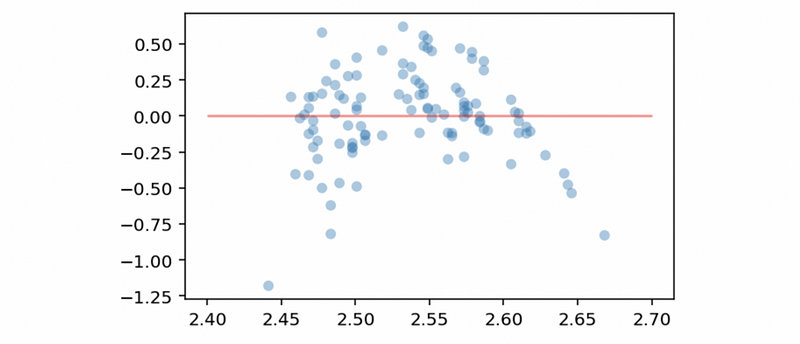
Now we can conclude that there’s no heteroscedasticity problem in this model based on this plot. However, there seems to be a linearity problem (non-linear) in this model. In order to eliminate this non-linear effect, we have to conduct an exponential calculation on the independent variable (we are going to explain in details later).

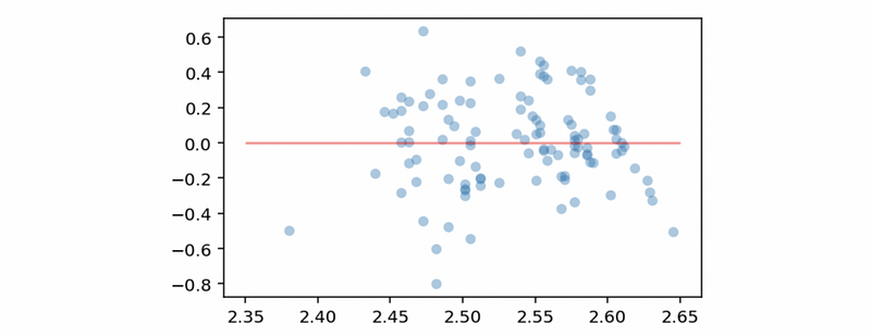
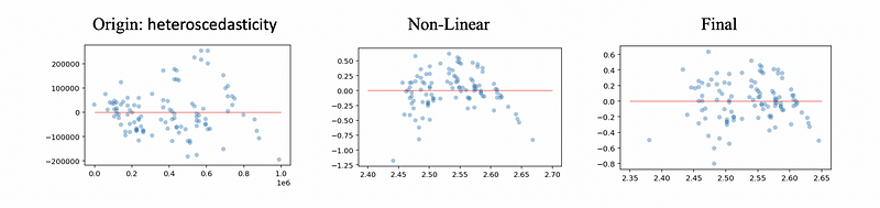
Let’s review what we have talked about by a brief summary,

b. Weighted Regression

Although the log transformation is easy to use, however, it has to be used only when the residual vs. fitted value plot has a “Funnel” shape. This is a relatively strong condition and you can image that most of the heteroscedasticity problems we meet can not satisfy this feature. Therefore, we have generate a more general solution for the heteroscedasticity problem. This general solution is called the weight regression (or the weighted least square regression).

For a heteroscedasticity problem, we can conclude that,

Suppose we define Σ as,

then,

Suppose we define a weight matrix,

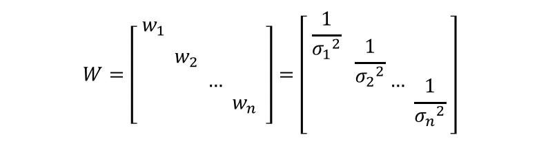
then the OLSE should be,

But how we can get the estimator W-hat of the weight matrix W? This is a tricky problem. A specific case of determining the value as follows,

When a plot of the residual against a predictor has a funnel shape, then we can fit the model of “ei² ~ xt”. Then use the fitted values of the model as the estimated variance. The example implementation code is,

c. Other Solutions (Not in details): generalized least squares, robust regression, or conducting the non-normality and non-linear solutions in the first place (sometimes, this can improve the heteroscedasticity problem as well).

Note that here’re the other topics that we are going to cover in the part 2:

• (5) Step 5. Check Normality
• (6) Step 6. Check Linearity
• (7) Step 7. Modify the initial model and fit the data again
• (8) Step 8. Best Subset Model Selection: based on adjusted R²
• (9) Step 9. Step-wise Model Selection: based on t-test
• (10) Step 10. AIC/BIC Method