Linear Regression 10 | Model Diagnosis Process for MLR — Part 2

Linear Regression 10 | Model Diagnosis Process for MLR — Part 2

1. Model Diagnosis Process for MLR

• (0) Goal of Modeling
• (1) Step 1. Check Multicollinearity
• (2) Step 2. Fit the Initial Model
• (3) Step 3. Check Influential Points
• (4) Step 4. Check Heteroscedasticity

You can find the topics above in part 1.

Now let’s continue our discussion.

(5) Step 5. Check Normality

• Reason: We have made an assumption of normally distributed error terms. As we have said in the SLR part, the normally distributed error terms assumption is a “strong” assumption so that it won’t affect the BLUE feature of the OLSE. Normally, the normality assumption is presented but it is described as a less important assumption compared with the other assumptions.

• Results:

a. The OLSE is still the best linear unbiased estimate (BLUE).

b. Normality is needed to perform t-test, confidence interval and the ANOVA. So if there’s no normality, then the inference can no longer work (However, there’s actually an exception because of the central limit theorm).

c. Because the central limit theorm tells us that if the sample size is large enough, then it’s distribution will turns out to be a normal distribution. We can say that when the sample size is large (empirically > 30), then the CLT guarantees that it’s approximately normally distributed. So that we can still use the perform t-test, confidence interval and the ANOVA.

• Detection

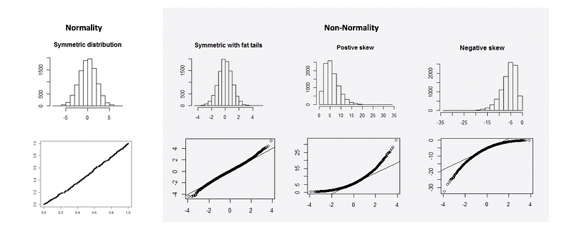
a. Q-Q Plot is a way to examine normality. If a QQ plot results in approximate linear on diagonal of its plot, then it suggests the normality.

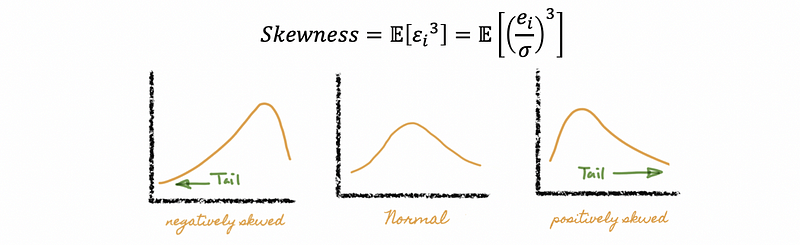
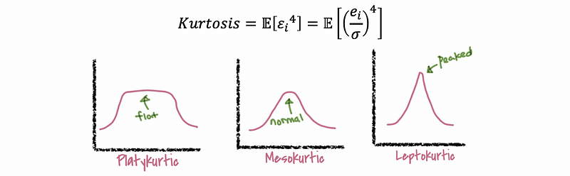
b. The Skewness and the Kurtosis also indicates a normality of the residuals. It will be helpful if you refer to the “moment” part of the following article.

And there’s also,

When σ for the error term is unknown, we can estimate this value by the sample variance of the residuals. Thus,

then,

Note that we have to detect both the skewness and the kurtosis for being zero in order to make a normality conclusion, or there will be a non-normality problem for the error terms.

However, it is always not accurate to use an approximate 0 as our evidence for normality. It’s a better idea if we can use a hypothesis inference to figure out our conclusion.

c. D’Agostino’s Omnibus K-Squared Normality Test

Suppose we define that,

Then the Omnibus K-Squared statistics is defined as,

Where Z1 and Z2 are two functions that we don’t have to know or understand them here, but this page may be helpful if you want to know more about these two functions.

Because the omnibus K-Square statistics follows the Chi-Square distribution (we don’t have to know the reason), then we can construct a hypothesis testing of it.

Then, because

Then we reject H0 if the p-value of this statistics is less than 0.05, this means that the normality of this model is not true.

d. Jarque–Bera Test

The Jarque-Bera test is another way to find out whether the error terms are normally distributed. It is quite similar to the D’Agostino’s Test. The null hypothesis and the alternative hypothesis of the JB test is,

Then the Jarque-Bera Statistics is defined as,

Then, because,

Then we reject H0 if the p-value of this statistics is less than 0.05, this means that the normality of this model is not true.

Note that the Jarque-Bera test is very sensitive to the outliers.

• Solutions

a. Natural-Log Transformation on y

To deal with the non-normality problem, first of all, we can try the natural-log transformation out,

We can use this method because the natural-log transformation can be used to make highly positively skewed distributions less skewed.

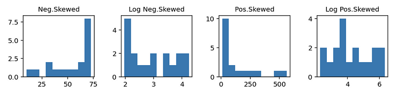
b. Box-Cox Transformation on y

Based on the log transformation, we can know that the log transformation works pretty well for the positively skewed data, while we have to make some change to the negatively skewed data (in the case above, we have to use 80-i). This is not convenient for us.

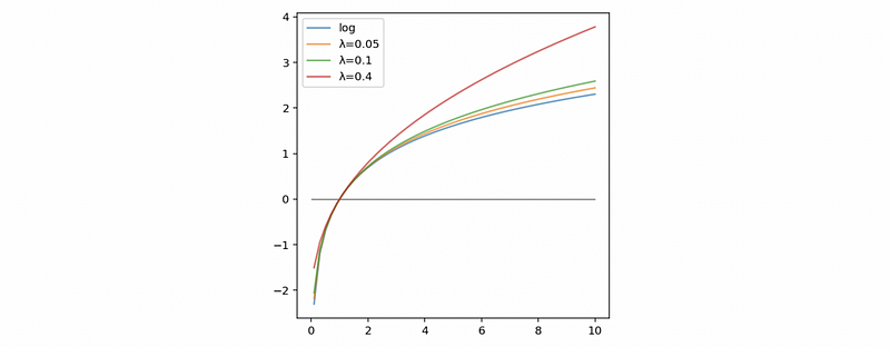
In fact, we want to construct a transformation that can work for both the positively skewed data and the negatively skewed data, then the answer of this kind of transformation is the box-cox transformation. It is defined as follows,

Why we can have this formula? Let’s think about what it will be like when λ is limited to zero. By L’Hôpital’s rule,

So when λ is close to zero, then the box-cox transformation will be approximatly equal to the natural-log transformation.

When λ is negative or positive, we can have two different forms of this transformation for the negatively skewed data and the positively skewed data, respectively,

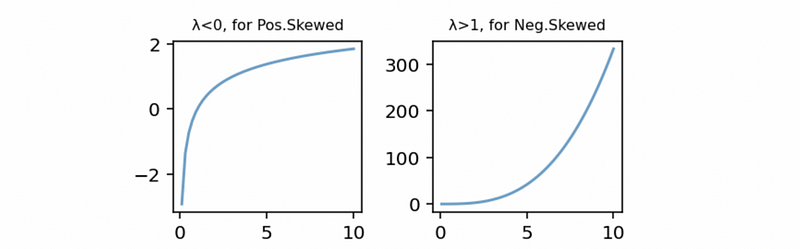
Then we redo the Box-Cox transformation for our case above and we can find out it also works for our data,

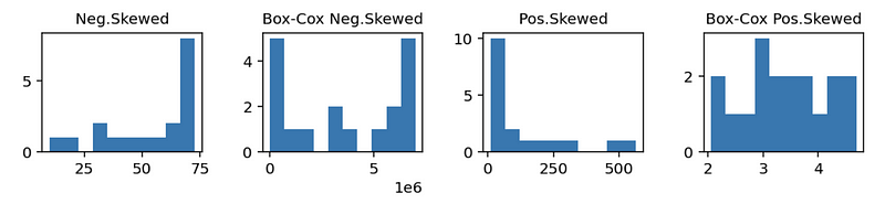
Okay, now here’s another question. How can we choose a proper λ for the Box-Cox transformation? Practically, we don’t have to calculate the proper lambda on our own, instead, we can call the stats.boxcox function in python to calculate a proper lambda for us.

from scipy import stats

y = [10,12,17,25,30,37,40,42,47,64,87,109,140,181,253,319,480,564]

fitted_data, fitted_lambda = stats.boxcox(y)
print('The fitted lambda is:', fitted_lambda)

The output is,

The fitted lambda is: -0.08379804288959128

This is quite close to what we have chosen (-0.1) in the previous case.

c. Collect more data! Because when the sample size is large, then the skewness of the data won’t impact the model estimation or inference too much.

(6) Step 6. Check Linearity

• Reason: When there is a non-linearity problem between the dependent variable and the independent variables, there can be two reasons. First, there may be some non-linear terms (i.e. squared terms). Second, there may be some interaction terms. Note that although there are many ways to adjust a non-linear model, we have to be extremely careful.
• Solution for Non-linear Terms

a. Nonlinear Approach: This is the most complicated way. By adding polynomial terms in MLR, it adds the number of the parameters and it can also adds the probability of multicollinearity. The cost for this approach is that all the testing methods can become unstable and invalid. Also, there will be no analytical expressions for the MLR estimation.

b. Log-log Transformation: it is a powerful tool because it will not lose any inference.

c. Transformation on x

• Solution for Interaction Terms

In practice, we only add interaction terms if we obtain the knowledge in advance that a significant interaction may exist in the study.

We will continue our discussion in part 3.

• (7) Step 7. Modify the initial model and fit the data again
• (8) Step 8. Best Subset Model Selection: based on adjusted R²
• (9) Step 9. Step-wise Model Selection: based on t-test
• (10) Step 10. AIC/BIC Method