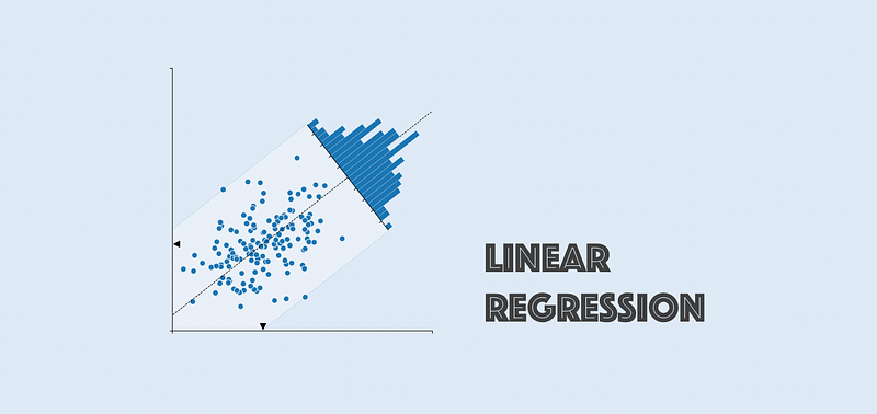
Linear Regression 12 | Model Diagnosis Process for MLR — Part 3
Linear Regression 12 | Model Diagnosis Process for MLR — Part 3
- Model Diagnosis Process for MLR
- (0) Goal of Modeling
- (1) Step 1. Check Multicollinearity
- (2) Step 2. Fit the Initial Model
- (3) Step 3. Check Influential Points
- (4) Step 4. Check Heteroscedasticity
- (5) Step 5. Check Normality
- (6) Step 6. Check Linearity
You can find the topics above in part 1 and part 2.
Let’s continue our discussion.
(7) Step 7. Modify the initial model and fit the data again
Because we have modified the data so that our data can be able to suit the assumptions of our linear model. Because we can put different variables as our predictors and this results in several linear models. We have to choose the best model so that our final model is the best model. This process is called the model selection process and we have quite a lot of measures to tell whether or not a model has a good performance.
(8) Step 8. Best Subset Model Selection: based on adjusted R² or Mallow’s Cp
- Criteria #1. R-Square

This is always not a good idea in MLR because it will say yes to the overfitted model. We have talked about this
- Criteria #2. Adjusted R-Square

The adjusted R-square takes a balance of the decrease in SSE and the decrease in the degree of freedom when adding more predictors, so it will have a better performance in telling the overfitted model.
- Criteria #3. Mallows’s Cp
Given a linear model with k parameters such as,

Suppose we select p parameters (p-1 predictors) from the full model, then the Mellows’s Cp statistic for this subset model is defined as,

We don’t have to know how to construct this statistic.
The most common interpretation of the Mallows’s Cp is that smaller Cp values are better as they indicate smaller amounts of unexplained error. If the model with p-1 predictors is a good model that can be useful, then its Cp should be small and the Cp statistic should be close to the value p. This is because the MSE for the full model is then close to the MSE of the subset model.
In practice, since Cp is a sample estimate, then it could be less than the value p. You may want to choose the smallest model for which Cp ≤ p is true, but there can be an overfitting problem if Cp is less than 1.
- Criteria #4. Unbiased Mallows’s Cp
The unbiased Mallows’s Cp (unbiased for the prediction risk R, and we don’t have to understand this) is defined as,

Then, replace the Cp with the definition of the Mallows’s Cp,

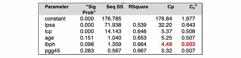
This measure is equivalent to the Mallows’s Cp with a different value. The similarity between the unbiased Mallows’s Cp and the Mallows’s Cp is that the smaller values are better in the model selection process. For example, here is a possible result we can have from a certain model.
(9) Step 9. AIC/BIC Method
- Why we have those two methods?
Both the Akaike Information Criterion (AIC) and the Bayesian Information Criterion (BIC) measures the amount of information lost by a given model. With the common sense that the less information a model loses, the higher quality the model has, we can select the model with those two criteria.
In summary, the smaller values of these two criteria indicate a better model.
- Recall: Likelihood Function
The likelihood function is the joint probability density of all the observations in the sample. It tells us the general probability we have to obtain such a certain sample. So that we want to maximize the likelihood of obtaining our sample in order to get the best-fitted parameters.
Because the density function of the Gaussian distribution is less than 1, then we are able to draw a conclusion that the maximized likelihood of the sample set is no more than 1 and thus, the maximized log-likelihood is negative.
- Akaike Information Criterion (AIC)
Suppose k is the number of parameters of a linear regression model, then let L-hat be the maximum value of the likelihood function for the model. The AIC is defined by,

We are having this result because of the information theory and we don’t have to understand it now. Note that the multiplier of the k is 2, which is defined as the penalty coefficient on the number of the parameters. In fact, AIC and Mallows’s Cp is equivalent mathematically.
- Bayesian Information Criterion (BIC)
AIC and BIC are theoretically different methods. AIC is a based on the likelihood function whereas BIC is based on the estimated function of a posterior probability of a model being true.
Although these two criteria are based on different assumptions, in practice, the only difference is in the size of the penalty. BIC penalizes the model complexity more heavily.

- Interpretation of the AIC and the BIC
A predictor has the lowest AIC and BIC means that the amount of information lost by removing this predictor from the model is minimum among all the predictors.
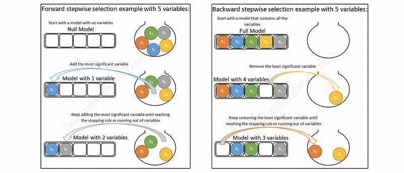
(10) Step 10. Stepwise Model Selection: based on t-test
There are two kinds of stepwise model selection. If we start will the null model with none of the predictors and we add 1 predictor in each step, then it is called a forward stepwise model selection (forward selection). If we start with the full model and we remove 1 predictor in each step, then it is called a backward stepwise model selection (backward selection).
- When to stop selection: by AIC and BIC
When we add more predictors to the model or we remove the predictors from the model, we have to set up a standard for our model so that we can know when to stop our selection. The first standard we can use is by AIC and BIC.
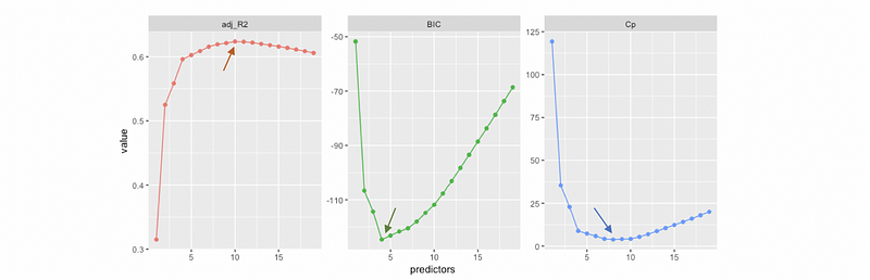
When the AIC and BIC for adding a new predictor is relatively low and the tendency is flat, then we are able to make the conclusion that the amount of information lost by this predictor is so small that we can stop our selection. For example, in the following picture, we are able to say that we can stop at the 4th predictor (the critical turning point) because it has the minimum AIC and BIC.

- When to stop selection: by Mallows’s Cp
Similar to AIC and BIC, the Mallows’s Cp can be used to find where to stop. Because a smaller Cp tells a better performance of the model, then we have to find the lowest Cp for our model.

- When to stop selection: by Adjusted R-Square
It is quite obvious that a higher adjusted R-Square tells a better performance of the model. Note that based on different criteria, the destination of the selection process can be different. For example,
- When to stop selection: by t-testing and F-testing
The t-testing and the F-testing process can also be used in the stepwise selection. But they are old-school methods and we don’t use them commonly nowadays.