Linear Regression 14 | Logistic Regression (Logit) and Probit Regression

Linear Regression 14 | Logistic Regression (Logit) and Probit Regression

1. Basic Settings of the Logistic Regression Model

The logistic regression model (aka. Logit model) is not a new concept. It is actually a specific SLR model. If the response variable (dependent variable) for SLR can take only the binary outcomes, then the SLR model will become a logit model.

It can also be clear that the response variable actually follows a Bernoulli distribution of Bern(πi), where πi is the probability that the response variable takes 1 as a result.

(1) From SLR to Logit

Suppose we have an SLR model as follows,

If you are not familiar with this, then you have to refer to,

Then, assume yi ~ Bern(πi),

Apply this property on the SLR model and then,

Here, we don’t use the strong assumption of the error term because the normality no longer holds for a logit regression (we will talk about it later). Instead, we will assume a zero mean for the error term,

Then,

Let’s now see the meaning of this model. Given a specific xi, then we can calculate a πi which is the probability that we can confirm that yi will be 1. If πi is zero, then we can conclude that it is not possible for yi to be 1, and while πi is 1, then we can 100% sure that yi will be 1. This model is called the probability linear model of the response variable and we can calculate the probability of yi = 1 with this model.

But, wait a minute. This is not a logit model, because we want to have a model that gives us the exact value of yi, not the probability of yi = 1. So we have to change this model a little bit to make it a logit model. Before we continue, let’s talk about the properties of the probability linear model.

(2) Probability Linear Model Properties

a. Error terms ϵi’s are also binary (Linear model)

We have removed the strong assumption of the SLR and we said that the strong assumption no longer holds for the probability linear model. This is because the error terms are also binary (not binary distributed, it actually means that the error term will take only two values given a specific xi).

Proof:

Given a specific xi,

This shows the two possible values for the error term.

b. No Error terms (Probability linear model)

Because the probability linear model is regressed on the probability, then under the assumption of zero means, the error terms will no longer exist.

c. OLSE is not the optimal estimate

For SLR, we have talked that the variance must be constant (not heteroscedastic) in order to have the conclusion that OLSE is the best estimate for the model. However, this can not hold anymore because the probability linear model must be a heteroscedasticity model.

Proof:

From what we have discussed,

Then, it is clear that the variance can be different for different observations.

d. Constraint on the results

Because the fitted values for the probability linear model should be probabilities. Then, they must meet the definition of the probability that the value of them should be between 0 and 1, or they will be meaningless. So here’s the constraint for the probability linear model which SLR doesn’t have,

How we can make this possible for us?

With,

We would like to find a function f that project the result to the range (0, 1), this kind of functions has a name called the sigmoid functions,

Practically, we can choose the following two sigmoid functions, the inverse logit function, and the inverse probit function.

(3) Logit Function

The CDF of the logistic function (typically, the logistic function we choose s = 1 and μ = 0 for a more specific expression) is defined by,

Then the inverse function of the logistic function is called the logit function.

(4) Probit Function

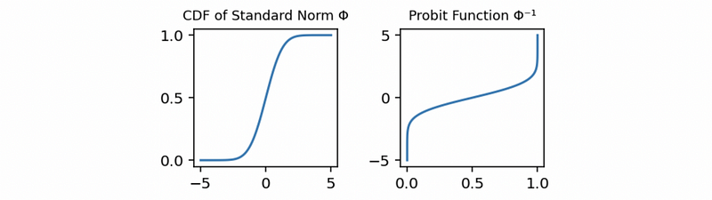
Suppose x follows the normal distribution N(0, 1) and its density function is,

Then the CDF function can be calculated by,

Then the inverse function of Φ is called the probit function.

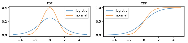
(5) Logit Function vs. Probit Function

By our discussions above, the probability linear model should finally be,

Then we can draw these two plots together to compare them,

(6) Model Selection

So when should we choose the logit model and when should we choose the probit model? This is based on our assumption of the error term of the original SLR model (we will see an example to understand what’s the meaning of this).

Now, let’s see an example. The first time moms, if left alone to go into labor naturally tend to be pregnant for about 41 weeks. If we suppose yi is the number of weeks that a mother i will give birth to a baby, and xi is the alcohol consumption in the period of pregnancy. Naturally, this is an SLR problem,

Now let’s say that we have a threshold of 38 weeks. If the baby is born in 38 weeks, then he/she is reckoned to be a preterm birth. However, If the baby is born after 38 weeks, then he/she is normal birth. The variable zi is defined as whether the baby of the mother i is prematurely birthed (value = 1) or normally birthed (value = 0).

Suppose πi is defined as the probability of getting a normally birthed baby. Then,

then,

then,

• Assume that the error term of the SLR is normally distributed, then,

this is to say that,

after standardization can be equivalent to,

where Z is standard normal distributed. Then,

then,

• Assume that the error term of the SLR is logistically distributed, then we will have the fact that (see the logistic distribution for more information),

then, because we also have,

Define the standardized error term as

then,

Because the “dagger” error term follows the standard logistic distribution, then,

then, this is also to say that,

We can see that the final result of probit and logit is actually the estimated (predicted) probability that the binary response variable = 1.

In practice, it can be hard to make the assumption that whether or not the error term is normally distributed or logistically distributed. We always choose the logit model because it is easier than the probit one.

2. Parameter Estimation

(1) Choosing Estimator

Because we have said that the OLS method is not the best for the logit (or probit) regression, then it can not be used to estimate parameters because there are no error terms.

(2) Maximum Likelihood Estimate

As we have discussed yet, the maximum likelihood estimate is the method to find the best parameter through maximum the result of the likelihood function, and the likelihood function is defined as the product of all the probability density of all the observations.

As our assumption goes,

Then for the i-th observation,

Then by the definition of the likelihood function,

then,

then, the log-likelihood function should be,

then,

By the fact that,

this is also,

then,

then,

then,

by equation (1) and (2),

this is also,

This is out log-likelihood function and we would like to maximize this in order to find the estimate,

In general, the maximum likelihood estimates are obtained by using the iterative algorithms, and we don’t have to calculate them manually.

(3) The Definition of Odds

In the logistic regression, the odds are defined as the estimated probability of success (value = 1) divided by the estimated probability of failure (value = 0). This is to say that,

Suppose we have already calculated the estimates by MLE as β0-hat and β1-hat, then,

then,

thus, the odd for observation i is also defined as,

(4) The Definition of Odds Ratio

The odds ratio (OR) is defined as the changing rate of odd for the observation i when the value of the predictor x increases by 1 unit. Mathematically, it is then defined as,

Then,

In conclusion, the odds ratio of the predictor x can be calculated by,

Note that this result holds for all the observations.

(5) Odds Ratio Interpretation

Because the odds ratio (OR) is defined as the changing rate of odd for the observation i when the value of the predictor x increases by 1 unit, it represents the multiplier of adding one unit.

Therefore,

• When the odds decrease when the value of x increase,

• When the odds increase when the value of x increase,

• When the odds remain the same when the value of x increase,

3. Multiple Logit Regression

The multiple logit regression is quite similar to the single logit regression. Of course, first of all, we can form an MLR model,

This is also,

Then, by multiple logit regression,

By MLE, the estimated probability for the i-th observation πi-hat is then,

The odd of the i-th observation is,

The odd ratio for the predictor p is,

where βp-hat is the parameter for the predictor p.

4. Logit Regression Prediction

(1) Threshold Probability

Because the logit regression or the probit regression will finally give a value of probability, suppose we want to tell whether or not the final result is a success (value = 1) or a failure (value = 0), we have to set a threshold probability π* that,

• if πi-hat ≥ π*, then the i-th observation is predicted to be a success (yi = 1)
• if πi-hat < π*, then the i-th observation is predicted to be a failure (yi = 0)

(2) Model Validation: Confusion Matrix

We can tell whether or not a logit model is good or not through a confusion matrix, which is defined as,

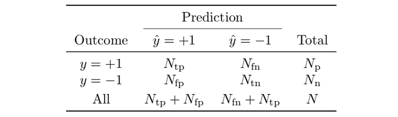
Where TP means true positive, FP means false positive, FN means false negative, and TN means true positive. In practice, the most common measure for a model is the true positive rate (or recall rate) and the Precision.

• Error Rate

• [IMPORTANT] True positive rate (also known as the sensitivity or recall rate)

• False positive rate (also known as the false alarm rate)

• Specificity or true negative rate

• [IMPORTANT] Precision

(3) Model Validation: Accuracy

The accuracy of the model is defined as the proportion of the true predictions (no matter true positive or true negative), then,

(4) Model Validation: Precision-Recall Linear Combination

A wiser way to consider which one is the best model is to make a combination of the recall rate and precision. The simplest one is to make a linear combination for these two values,

where c1 and c2 are two constants chosen by us.

(5) Model Validation: F-Score

A more commonly used measure is the combination of recall and precision. This is called the F-Score or F-Measure (this is nothing related to the F statistic of the inference).