Operating System 16 | OS Scheduling, First-Come&First-Serve, Shortest-Job First, Preemption…

Operating System 16 | OS Scheduling, First-Come&First-Serve, Shortest-Job First, Preemption, Priority, Timeslicing, Runqueue, Linux Scheduler, and Scheduling on Multi-CPU Systems

1. Introduction to OS Schedular

(1) The Definition of Tasks

In this section, we will use the term tasks to interchangeably mean either processes or threads.

(2) The Definition of the Scheduler

The CPU scheduler is a process that decides how and when the tasks access the shared CPUs. The scheduler considers both the ULPs and ULTs as well as the KLTs.

(3) CPU Scheduler Functions

Recall this figure we used when we talked originally about the processes and process scheduling,

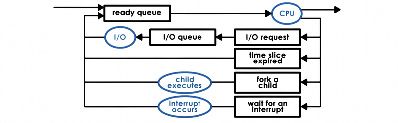
the responsibility of the CPU scheduler is to,

• When the CPU becomes idle, choose one of the tasks in the ready queue (which is implemented by a runqueue data structure)
• The scheduler dispatches this task onto the CPU. This means that it will perform a context switch, enter the user mode, set the PC appropriately, and we are ready to execute this task on the CPU.

Tasks may become ready in the ready queue so they may enter the ready queue after,

• an I/O operation they have been waiting on has completed
• they have been woken up from a wait for an interrupt
• when somebody has forked a new thread
• the tasks with their time slice expired

(4) Three Options for Task Selection

For an OS scheduler, the choices of how to schedule are analyzed in terms of tasks. These are being scheduled onto the CPUs that are managed by the OS scheduler. Basically, we can have three options to handle tasks,

• Assign tasks immediately: for an OS scheduler, we can choose a simple approach to schedule tasks in a first-come, first-serve (FCFS, aka. FIFO) manner. This is quite simple and we don’t have to spend overheads on the scheduler itself.
• Assign simple tasks first: the OS scheduler can also assign or dispatch simple tasks first. The outcome of this kind of schedule can be that the throughput of the system overall is maximized. The schedulers that actually follow this kind of algorithm are called shortest-job first (SJF) schedulers.
• Assign complex tasks first: the OS schedular can also assign or dispatch complex first. The goal of the scheduler is to maximize the utilization of all the resources of the system (e.g. CPUs, memory, other devices, etc.).

(5) Scheduling Performance

Since we will be talking about different scheduling algorithms, it will be important for us to have some metrics. These meaningful metrics include

• throughput
• the average time it took for tasks to complete
• the average time that tasks spent waiting before they were scheduled
• the overall CPU utilization

We will use some of these metrics to compare some of the algorithms that we will talk about.

2. Run-to-Completion Scheduling

(1) Run-to-Completion Scheduling

The run-to-completion scheduling assumes that as soon as a task is assigned to a CPU, it will run until it finishes or until it completes. For this scheduling, we will have the following assumptions,

• we have a group of tasks we have to schedule
• we know exactly how much time these tasks need to execute
• no preemptions/interrupts in the system
• single CPU

(2) Algorithm #1: First-Come, First-Serve (FCFS)

The first and simplest algorithm we are going to discuss is the first-come, first-serve (FCFS) algorithm. In this algorithm, tasks are scheduled on the CPU in the same order in which they arrive, regardless of their execution time, of load in the system, or anything else.

Whenever a new task becomes ready, it will be placed at the end of the run queue. Then whenever the scheduler needs to pick the next task to execute, it will pick from the front of the queue.

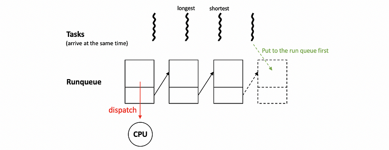
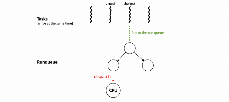
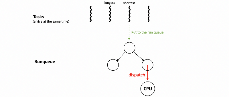
(3) Algorithm #2: Shortest-Job First (SJF)

Another algorithm that’s called Shortest Job First (SJF) and the goal of this algorithm is to schedule the tasks in the order of a short-to-long execution time sequence. This schedular can be implemented by a balanced tree instead of a queue because it will not follow the FIFO rule. We can also use an order queue that sorts the elements every time a new task is put in the queue, but this will be more complex than a balanced tree.

(4) Algorithm #3: Complex First

We can also call the most complex one first so as to make full use of the system resources.

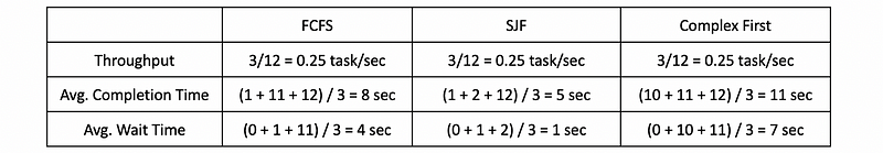
(5) Scheduling Performance for Algorithms: An Example

Now, let’s see an example about the performance of these algorithms. Suppose we have three tasks T1, T2, and T3, which have the following execution time,

T1 =  1 s
T2 = 10 s
T3 =  1 s

Let’s assume that they will arrive in the order of T1 -> T2 -> T3 so that the performance of the three algorithms will be,

3. Preemptive Scheduling

(1) The Definition of Preemptive Scheduling

So far in this discussion, we assumed that a task that’s executing on the CPU cannot be interrupted or preempted. Let’s now relax that requirement and start talking about preemptive scheduling, in which the tasks don’t hog the CPU until they’re completed.

(2) SJF + Preemption With Execution Time

Now, let’s see an example of preemption scheduling with the SJF algorithm. The T1 and T3 thread will arrive 2 seconds after T1 arrives. Thus, we can have,

Task         ExeTime        ArrTime
------       ---------      ---------
T1           1              2
T2           10             0
T3           1              2

Because T2 arrives first, it will be executed in the first place. However, when T1 and T3 arrive, they will be preempted and scheduled to T1 and T3 because we have to follow the SJF algorithm. When T1 and T3 complete, we can take the remaining time to execute T2. Thus, the execution chart will be,

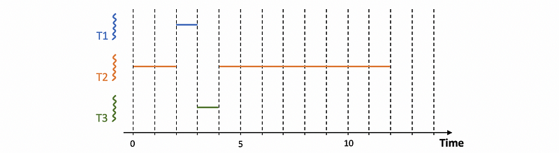
So basically what would happen is whenever tasks enter the run queue like T1 and T3, the scheduler needs to be invoked. So it can inspect the execution times, and then decide whether to preempt the currently running task (T2) and schedule one of the newly ready tasks.

(3) SJF + Preemption Without Execution Time

So far we talked as if we know the execution time of the task, but it’s really hard to claim that we know the execution time of a task. It depends on a number of factors, for example,

• the inputs of the task
• whether the data is present in the cache or not
• which other tasks are running in the system
• etc.

Therefore, we have to use some kind of heuristics in order to guesstimate what the execution time of a task will be and history is a good predictor of what will happen. For instance, we can think about,

• Point Estimate: how long a task ran the very last time it was executed?
• Windowed Average: how long a task ran the last N time it was executed on average? The windowed average means

So we compute some kind of metrics based on a window of values from the past and use that average for the prediction of the behavior of the task in the future.

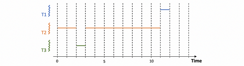
(4) SJF + Preemption With Priority

SJF Priority is another way to decide how to schedule tasks and when to preempt a particular task, and tasks that have different priority levels, that is a pretty common situation. For instance, several operating system-level threads run OS tasks that would have higher priority than other threads that support by ULPs. With priorities, the schedulers will have to run the task with the highest priority in the first place. It is clear that preemption will be needed for this implementation. This scenario is also called priority scheduling.

Now, let’s see an example.

Task         ExeTime        ArrTime       Priority
------       ---------      ---------     ----------
T1           1              2             P1
T2           10             0             P2
T3           1              2             P3

In this particular example, the priorities P1, P2, and P3 are such that the first thread P1 has the lowest priority. Again, we start with the execution of T2 since it’s the only thread in the system. However, when T1 and T3 become ready at time 2, we will look at the priorities and see that T3 has the highest priority. So when threads T1 and T3 are ready, T2 is preempted and the execution of T3 will start. When T3 completes, T2 starts running again, and then T1 will have to wait until T2 completes to start.

If the scheduler needs to be a priority-based scheduler, it will somehow need to quickly access the priorities and the execution context in order to select the one that has the highest priority to execute next.

(5) Priority Scheduling Implementation

To implement priority scheduling, we can have multiple run queue structures for each priority level. And then have the scheduler select a task from the run queue that corresponds to the highest priority level.

Another option is to have some ordered data structures like the balanced tree that we have discussed.

(6) Priority Scheduling Danger #1: Starvation

Basically, there can be a possible danger called starvation if we want to have priority scheduling. Starvation means that a low priority task can be stuck in a run queue just because there are constantly higher priority tasks show up in some of the other parts of the run queue.

One mechanism that we use to protect against starvation is so-called priority aging, which means that the priority of the task isn’t just a fixed priority. Instead, it is a function of the actual priority and the time spent in the run queue.

The idea is that the longer a task spends in a run queue, the higher the priority should become. So eventually, the task will become the highest priority task in the system and it will run. In this manner, starvation will be prevented.

(7) Priority Scheduling Danger #2: Priority Inversion

An interesting phenomenon called priority inversion happens once we introduce locks into the scheduling. In the following diagram, suppose the priority is: T1 > T2 > T3 and T3 acquires a mutex lock in the first 3 seconds without unlocking. Note that task T1 will also require this lock at time 7, so it will be blocked since T3 holds the lock.

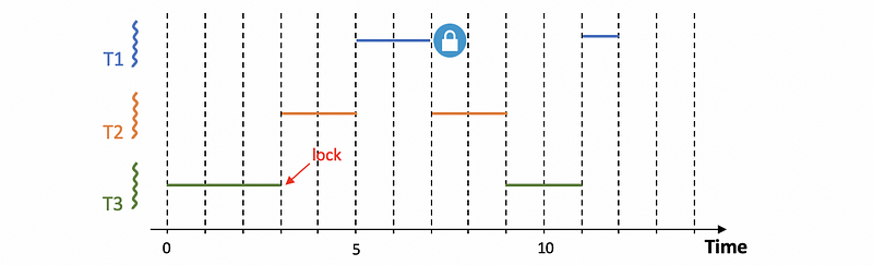
A solution to this problem is to temporarily boost the priority of the mutex owner. This means that when the highest priority thread needs to acquire the lock that’s owned by a lower priority thread, the priority of T3 is temporarily boosted to be basically at the same level as T1. This technique can be used to keep track of who is the current owner of the mutex.

Obviously, if we are temporarily boosting the priority of the mutex owner, we should lower its priority once it releases the mutex. This is a common technique that’s currently present in many operating systems.

4. Round Robin (RR) Scheduling

(1) Round Robin Without Time slicing

In practice, we can hardly tell how much time we need form executing a task, especially when there’s an I/O operation. But in the previous discussions, we have assumed that we know the executing time for each task. The round-robin scheduling can be used when we don’t know the execution time for each task and we will conduct a context switch when we have to wait for an I/O operation.

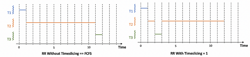
Let’s see an example. Suppose we have 3 tasks arrive at time 0. Each of them has an execution time of 2 seconds. However, task T1 has to conduct an I/O operation and it has to wait from time 1. The I/O operation of T1 is supposed to finish in 2 cycles, but because we don’t assign a priority in this case, the task T1 will have to wait for time 3 to continue.

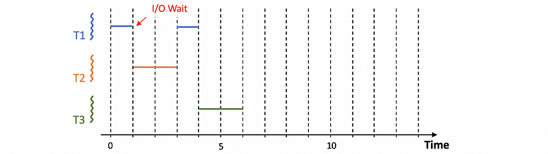
So what if we assign priorities for this case? Let’s suppose that we have priority T3 > T2 > T1. In order to implement priorities, we also have to include preemptions.

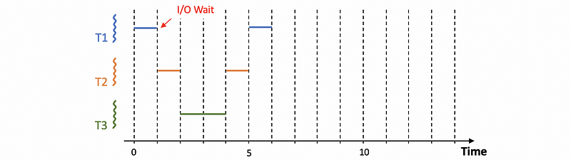
If T2 and T3 have the same priority higher than T1, we will have,

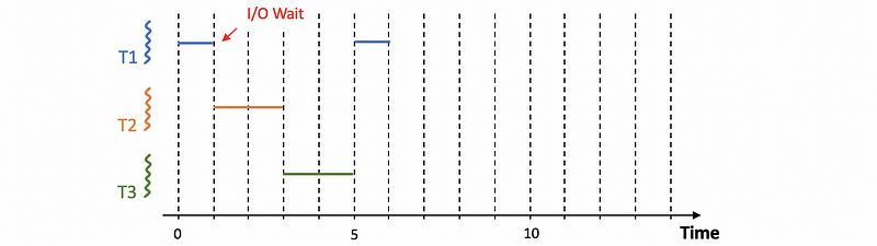
Note that when we haven’t got any I/O operations, the RR schedule will be exactly the same as the FCFS.

(2) The Definition of Time slicing

Further modification made for Round-robin scheduling is not waiting for tasks to yield explicitly. Instead, we would interrupt them by mixing the tasks that are in the system at the same time. This mechanism is called time-slicing. For example, we can give each task a time slice of one time unit (when there are no priorities), and then we will have,

A time slice (aka. time quantum) is the maximum amount of uninterrupted time that can be given to a task. Based on the definition, a task can actually run less amount time than what the time slice specifies, especially for the case when there is,

• I/O operations
• synchronization (e.g. mutex, cv, etc.)

The tasks that use timeslices are interleaved, which means that they are time-sharing the CPU. For CPU-bound tasks, time slice is the only way we can achieve time sharing. They will be preempted after some amount of time specified by the time slice and we will schedule the next CPU-bound task.

(3) Timeslicing Performance

Let’s now use an example to see the performance of the time-slicing. Suppose we have the following non-priority tasks,

T1 =  1 s
T2 = 10 s
T3 =  1 s

Then we can draw the diagrams of when we have a RR scheduling without time-slicing (exactly the same as FCFS) and when we have a RR scheduling with time slides of 1 unit,

Then the performance of these two situations will be,

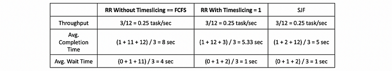
We can find out that even without knowing the execution time, we can also achieve a performance that is close to SJF based on the RR scheduling with time-slicing.

(4) Timeslicing Evaluation

There are really some benefits of using the time-slicing when the time slice is relatively short,

• no need for execution times
• short tasks finish sooner
• achieve a schedule that is more responsive
• I/O operations can be executed and initiated as soon as possible

The downside is that,

• more pure overheads for interrupting the running task, running the scheduler, and performing the context switch

Because of these overheads, in practice, the throughput will go down, the average waiting time goes up, and the average completion time goes up.

So as long as the time slice values are significantly larger than the context switch time, we should be able to minimize these overheads. In general, we should consider both the nature of the tasks as well as the overheads in the system when determining meaningful values for the time slice.

(5) Determining the Time Slice

We have seen that we can have a better performance if we have a shorter time slice because the scheduler can then become more responsive. However, we can also have significant overheads when the time slice is too short. Therefore, we have to make a balance between these two to get a proper length of the time slice. To find this properly balanced value, we have to look at two different scenarios in the next place.

• For I/O-Bound tasks: means that these tasks are mostly running for I/O operations
• For CPU-Bound tasks: means that these tasks are mostly running on the CPU without I/O operations

(6) Determining the Time Slice: For CPU-Bound Tasks

In summary, a CPU-bound task prefers a larger time slice (ts). Let’s see why by example.

Suppose we are given 2 CPU-bound tasks T1 and T2 with 10-sec execution time each. Assume the context switching time is 0.1 sec. Then, for the case when we have 1-sec time slice, 5-sec time slice, or ∞ sec (also means without) time slice, we can have the following diagram,

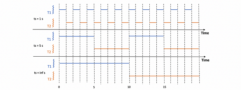
Thus, the performance will be,

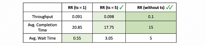
From this table, we can know that because CPU-bound tasks care more about the throughput and the average completion time, and they care less about the average wait time, the performance of these tasks will be better if we have a larger time slice. What’s more, it will be even better when we don’t have time slices.

(6) Determining the Time Slice: For I/O-Bound Tasks

One conclusion we can make is that for only I/O bound tasks, the value of the time slice is not really relevant. Let’s see an example.

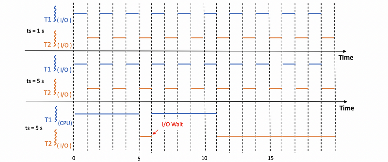
Suppose we have 2 tasks T1 and T2 and each of them takes 10 seconds for execution. The context switching time is 0.1 seconds and the I/O operations are issued every 1 second with each I/O operation completes in 0.5 seconds.

We can see from the following diagram that if both T1 and T2 are I/O bound tasks, we will get exactly the same performance because the current task will be interrupted for RR scheduling. However, when only T2 is I/O-bound with a CPU-bound T1, the performance can be different because T1 can keep executing because there will be no interrupts for I/O waiting.

Thus, in general, the performance will be,

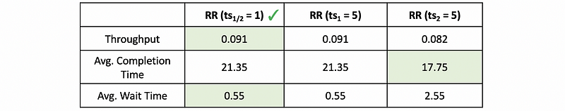
In this case, although the average completion time will be better, we would finally choose a smaller time slice.

(7) Timeslice Length Summary

CPU-bound tasks prefer longer time slices. The longer the time slice, the fewer context switches that need to be performed. So that basically limits the context switching overhead that the scheduling will introduce. Also, longer time slices keep the CPU utilization and throughput high.

I/O bound tasks prefer shorter time slices. This allows I/O bound tasks to issue I/O operations as soon as possible and, as a result, we achieve both higher CPU and device utilization as well as the performance that the user perceives that the system is responsive and that it responds to its commands and displays output.

(8) CPU Utilization Calculation

When we need to calculate the utilization of the CPU, we can use the following formula.

And we should follow the steps,

• Determine a consistent, recurring interval
• In the interval, each task should be given an opportunity to run
• During that interval, how much time is spent computing? This is the cpu_running_time
• During that interval, how much time is spent context switching? This is the context_switching_overheads
• Calculate

5. Runqueue Data Structure

(1) Assigning Different Lengths of Time Slices

If we want the I/O or CPU bound tasks to have different time slice values, we have two options,

• Maintaining the same runqueue data structure for both the I/O and CPU-bound tasks. Then we do classifications for telling whether this is an I/O-bound task or a CPU-bound task, and with the result of that, we can assign different time slices for each type.
• Maintaining two different runqueue data structures for I/O and CPU-bound tasks respectively. With each run queue, we will associate a different kind of policies that suitable for this kind of task that it is related with.

(2) Multiqueue Data Structure

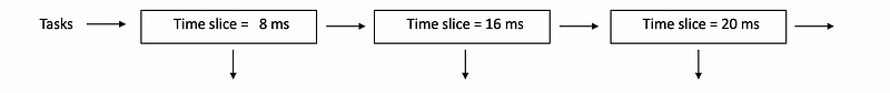
Now, let’s see the implementation of a multi-queue runqueue data structure. Suppose we have three runqueues in the system each of them will be assigned for different lengths of time slices (e.g. 8 ms, 16 ms, or 20 ms),

Based on the discussions above, the CPU-bound tasks tend to perform better when we have a longer time slice, while the I/O-bound tasks tend to perform better when we have a shorter time slice. Then we will conduct a classification of the tasks before we enter these runqueues.

• The most I/O intensive tasks will be assigned to the 1st queue (ts = 8 ms)
• Medium I/O intensive tasks will be assigned to the 2nd queue (ts = 16 ms)
• CPU intensive tasks will be assigned to the 3rd queue (ts = 20ms). Because the time slice for CPU intensive tasks is quite long, we can

The benefits that can be gained from these tasks will be,

• Time slicing benefits provided for I/O-bounds tasks
• Time slicing overhead avoided for CPU-bounds tasks

The downside is that,

• It can be hard for us to know whether we have an I/O-intensive bound

(3) Task Classification

It can be a problem for us to decide how I/O intensive of a task. We can use,

• history-based heuristics

But this can be even more complex when we have new tasks or some tasks that will change the behavior during the execution.

In order to deal with all these problems, Fernando Corbato developed the multi-level feedback queue data structure along with other work on the time-sharing system. He is awarded Turing Award because of this in 1990.

(4) Multi-Level Feedback Queue (MLFQ)

The idea of the multi-level feedback queue (MLFQ) is quite simple. Instead of classifying the task types all the time and this is quite complicated, we will decide not to do any classifications.

To deal with these problems, we will treat these three queues not as three separate run queues but as one single multi-queue data structure as follows,

This data structure can be used as follows,

• Step 1. Tasks enter the topmost queue. This queue has the lowest time slice and we are expecting that the I/O-bound tasks are the most demanding task and we would be a benefit from the context switching.
• Step 2. If the task stops executing before 8 ms, then this means that we made a good choice. The task will be kept at this level.
• Step 3. If the task used up the entire 8 ms time slice, this means that this task is more intensive on the CPU. So we will push it down to a lower level with a 16 ms time slice.
• Step 4. If the task used up the entire 16 ms time slice, this means that this task is more intensive on the CPU. So we will push it down to a lower level with a 20 ms time slice.
• Step 5. If the task in the low queue has an I/O wait, it will have a priority boost when it is released.

6. Linux Scheduler

(1) Linux Scheduler Example: O(1) Scheduler

The Linux has a scheduler called O(1) and we will talk about it next. It’s like a multi-level feedback queue with 60 levels, and also some things feedback rules that determine how and when a thread gets pushed up and down these different levels.

The O(1) scheduler receives its name because it’s able to perform task management operations such as selecting a task from the run queue or adding a task to it in constant time.

(2) Numeric Priority Numbers

The O(1) scheduler has 140 priority levels with 0 being the highest (ts = 100 ms) and 139 (ts = 10 ms) is the lowest. The priority levels can be grouped into two classes,

• 0~99: real-time tasks
• 100~139: time-sharing class

Each of the ULPs has one of the time-sharing priority levels,

• default priority: 120
• nice value: -20 ~ 19.

(3) Sleep Time and Priority

The time slice value will depend on the priority and the feedback from the sleep time.

• longer sleep time: means that the task needs interactive. So when longer sleep time is detected, we will boost the priority by reducing the priority by 5.
• smaller sleep time: means that the task is more compute-intensive. So we lowered the priority by reducing the priority by 5.

(4) Active Array and Expired Array

The runqueue in the O(1) scheduler is organized as 2 arrays of tasks.

When a task first comes into the run queue or active, it will be put at the back of the active arrive array corresponding to its priority value. When the CPU becomes available, the scheduler will select and pick up the next task from the active array to run with a constant time. The remaining tasks will be left in the queue and wait until their time slices expire.

When the time slice of a task is expired, this task will be inactive and it will be put into the expired array. When there are no more tasks in the active array, the pointers of these two lists will be swapped. As a result, the expired array can become the new active one and the tasks in it can be executed again.

(5) Problems for O(1) Scheduler

The O(1) was first introduced in the Linux kernel 2.5 by Ingo Molnar. In spite of its really nice property of being able to operate in constant time, the O(1) really affected the performance of interactive tasks significantly. As the workloads changed, as typical applications are becoming more time-sensitive (skype, movie streaming, gaming) the jitter that was introduced by the O(1) scheduler was becoming unacceptable. For O(1) schedulers, there can be 2 problems,

• Performance of Interactive Tasks: tasks that are put on the expired list will not be rescheduled until the array switches. As a result, the performance of the interactive tasks will become worse
• Fairness: fairness means that in a given time interval, all of the tasks should be able to run for an amount of time that is proportional to their priority. A lack of fairness means that even though there are multiple formal definitions of fairness, and O(1) doesn’t make any fairness guarantees

For that reason, the O(1) scheduler was replaced with the completely fair scheduler CFS and it became the default scheduler in kernel 2.6.23. Ironically, both of these schedulers are developed by the same person. Both the O(1) and CFS scheduler are part of the standard Linux distribution. CFS is the default. But you can switch to O(1) scheduler to execute your tasks.

(6) Linux Completely Fair Scheduler (LCFS)

The CFS is used after Linux kernel 2.6.23 and it is the default scheduler for all the non-real-time tasks. The main idea of a CFS is that it uses a red-black tree (aka. balanced search tree) and the red-black tree belongs to dynamic tree structures. The tree will be self-balanced as nodes are added or removed from the tree. We will not discuss this data structure in detail because it is beyond the scope of this series. But you should know that CFS always schedules the task which has the least amount of time on the CPU so that typically would be the leftmost node in the tree.

7. Scheduling on Multi-CPU Systems

(1) Computer Architecture Details

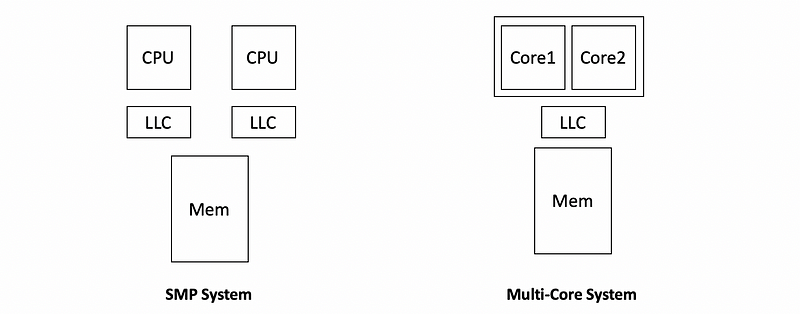
Before we discuss the scheduling in the multi-CPU systems, we have to know something about the architecture. The shared memory can be accessed by all the processors and these processors are called the shared memory multi-processors (aka. SMPs). Each of the processors has its own caches (e.g. L1 cache, L2 cache, etc.) and the last level cache (aka. LLC) may or may not be shared among the CPUs. There is a system memory called dynamic random-access memory (aka. DRAM) that is shared among all the processors. We will assume that in the following case, we only have one memory component, but it’s possible that there are multiple memory components in reality.

However, in the current multicore world, there can be some differences from the SMP system. In general, the common differences are,

• each CPU can have multiple cores
• each core can have private caches
• the entire CPU will share a single LLC

You can refer to the following picture for more insights,

Nowadays, it’s more common to have 6 or 8 cores for PCs in order to have multiple CPUs. We will discuss the following topics based on the SMP system because the multi-core system is quite similar and the same stuff can be easily applied.

(2) Cache-Affinity and Solution

The cache affinity happens because the processors have private LLCs in an SMP system. If a task has been run on one CPU, then we switch the execution of it on another CPU, we will probably meet a cold cache problem. If we assign this task to the same CPU, instead, we will have a cache hit which improves the performance. That’s why we have this cache affinity issue. To achieve this cache affinity, we have to keep tasks on the same CPU as much as possible.

We can implement cache affinity by the hierarchical scheduler architecture where at the top level, a load balancing entity in the scheduler divides the tasks among the CPUs. Then a per CPU scheduler with a per CPU run queue repeatedly schedules those tasks on a given CPU as much as possible.

The top-level entity in the scheduler can look at information such as

• the length of each of these queues
• whether a CPU is idle

to decide how to balance tasks among these CPUs.

(3) Non-Uniform Memory Access Platforms (NUMA)

In addition, it is also possible to have multiple memory nodes. However, the CPU and the memory nodes will be interconnected via some type of interface. For example, for modern intel platforms, there is an interconnect quick pipe interconnect (aka. QPI) that is used to connect the CPU with a memory. If that is the case, the access from a CPU to one memory node can be fast, but the CPU to the other memory node can be slow.

So it is clear that, from a scheduling perspective, it makes sense if the tasks are bound to those CPUs whose memory nodes are close to the state of those tasks. We call this type of scheduling NUMA-aware scheduling.

(4) Hyperthreading

If we use hardware to implement multi-threads, we can have hyperthreading (aka. hardware multithreading, chip multithreading, CMT, simultaneous multithreading, SMT). One way this has been achieved is to have multiple sets of registers. The context switching between hyper-threads is very fast because nothing has to be saved or restored and the CPU just needs to switch from using this set of registers to another set of registers.

One of the features of today’s hardware is that you can enable or disable this hardware multithreading at boot time. If it is enabled, each of these hardware contexts appears to the OS scheduler will be treated as a separate virtual CPU. In that way, when there is a memory I/O that can cost much longer than the cost of a context switch, which is almost 0 cycle in this case, the context on the CPU will be switched to another hyper thread. Therefore, hyperthreading can also hide memory access latency.

(5) Scheduling on Hyperthreading Platforms: Assumptions

The following discussion will be based on Fedorova’s paper named Chip Multithreading Systems Need a New Operating System Scheduler. Let’s first see the basic assumptions of this paper,

• a thread can issue an instruction on every single cycles, so the maximum IPC will be 1
• the memory access takes 4 cycles
• time for context switch between hardware is instantaneous
• we have an SMT system with 2 hardware threads

(6) Scheduling on Hyperthreading Platforms: 2 Compute-Bound Tasks

Now, let’s see the first case. Suppose that both of the hyperthreads are compute-bound, which means that they are both intensive to the CPU. However, given that there is only a CPU pipeline, only one of them can execute at any given point of time. As a result, these threads will interfere with each other and contend with the CPU pipeline resources. In the best case, every one of them will basically spend 1 cycle idling while the other thread issues its instruction. You can see this from the following diagram where C means compute and X means idle.

As a result, for each of the threads,

• the performance will degrade by 2
• the memory controller is idle

(7) Scheduling on Hyperthreading Platforms: 2 Memory-Bound Tasks

Now, let’s see the second case. Suppose that both of the hyperthreads are memory-bound. Because we have to wait 4 cycles to return from the memory, we can have 2 cycles that are unused for every 4 cycles. Now the diagram would be,

This strategy leads to some bad results because we are wasting the CPU cycles.

(7) Scheduling on Hyperthreading Platforms: 1MB-1CB Tasks

The final option is to consider mixing some CPU-intensive threads and memory-intensive threads. As a result, we end up fully utilizing each of the CPU cycles, and whenever there is a thread that needs to perform a memory reference, we context switch to that thread in the hardware and then context switch back to the CPU-intensive thread. Now the diagram would be,

This option is perfect because it

• avoids/limits the contention on the processor’s pipeline
• all the CPU and memory are well utilized

(8) CPU-Bound Tasks or Memory-Bound Tasks: by Counters

Well, we finally come to this question if we want to implement the scheduling above. The answer is to use a history-based counter. It is not convenient for us to use the sleep time and you can think about why. Fortunately, many hardware counters (e.g. L1, L2, LLC, power and energy data, etc.) can provide us useful information to decide whether it is a CPU-bound or a memory-bound task. In addition, there are also a number of interfaces that can be used for us, for example, the Oprofile and the Linux perf tool.

For instance, schedulers can look at LLC misses, and using this counter as a scheduler that can decide whether it is memory-bound or compute-bound. Or the same counter can also tell the scheduler that something changed in the execution of the thread so that now it is executing with some different data in a different phase of its execution, or maybe it is running with a cold cache.

In addition, most modern processors will,

• typically use multiple counters
• use some models for a specific architecture
• be trained based on well-understood workloads

(9) IPC as a Good Counter

Fedorova observes that a memory-bound thread takes a lot of cycles to complete the instruction therefore it has a high CPI. Whereas a CPU-bound thread will complete an instruction every cycle or near that and therefore have a CPI of one or a low CPI. She speculates that it would be useful to gather this type of information this counter about the cycles per instruction and use that as a metric in scheduling threads on hyperthreaded platforms.

Given that there isn’t an exact CPI counter on the processors that Fedorova uses in her work and computing something like 1/IPC would require software computation so that wouldn’t be acceptable.

For that reason, Fedorova uses a simulator that supposedly the CPU does have a CPI counter, and then she looks at whether a scheduler can take that information and make good decisions. Her hope is that if she can demonstrate that CPI is a useful metric, then hardware engineers will add this particular type of counter in future architectures.

(10) Experimental Information for Fedorova’s Paper

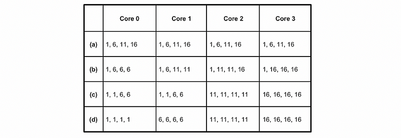
In order to prove that IPC is a good metric in the future, Fedorova designs an experiment and simulates the results. Here are some basic information about this experiment,

• 4-core 4-way SMT system (totally 16 hardware context)
• the synthetic workload with CPI of 1, 6, 11, 16
• 4 threads of each kind of CPI
• the metric should be IPC and its maximum value can be 4

Then the following experimental table is designed. She designed 4 experiments a, b, c, and d. And within each of these experiments, she assigned different workloads for each core.

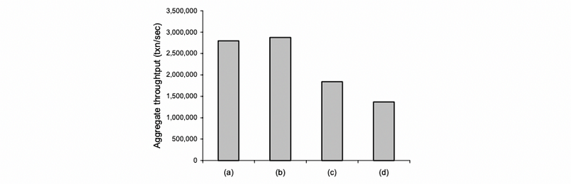
(11) Experimental Results for Fedorova’s Paper

So here is the final result. Because we have discussed that with a mixed CPI, we can result in better performance, the experiments a and b must have better performance than experiments c and d. If we look at c and d, the core 2 and core 3 of them will only be compute-bound or memory-bound and this is not good for us.

(12) Realistic Workloads

Although in the paper, it can be quite good for us to use the IPC metric as a metric, it is not the case in reality. Let’s see the following tables.

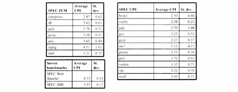
We can find out that all the common applications have a CPI of around 2.5 ~ 4.5, and these are exactly different from the synthetic workload of 1 ~ 16 that we mentioned in the paper. Therefore, the idea of using IPC as a scheduling metric will not be useful for a real workload.

In fact, the LLC will be a better counter in reality but we will not explain why in this series because it is beyond the scope.