Operating System 17 | Memory Management, Pages and Page Tables, Segmentation, Memory Allocation, …

Operating System 17 | Memory Management, Pages and Page Tables, Segmentation, Memory Allocation, Copy-On-Write, and Checkpointing

1. Introduction to Memory Management

(1) Virtual Addresses Vs. Physical Addresses

We have discussed that almost every application uses virtual addresses (VA) and these virtual addresses are translated to actual physical addresses (PA) in the physical memory (DRAM) where the particular state is stored. In fact, the virtual address space can be much larger than the physical address space.

(2) The Goal of Memory Management

In order to manage the physical memory, the OS must then be able to allocate physical memory and also arbitrate how it’s being accessed.

• Allocation: requires that the OS tracks how physical memory is used and also which frame is free among the physical memory. In addition, OS must have mechanisms to decide how to replace the contents that are currently in physical memory with the needed content that’s on some temporary storage like the disk.
• Arbitration: requires that the OS is quickly able to interpret and verify memory access. That means that when looking at a virtual address, the OS should be able to translate the virtual address into a physical address rapidly and verify that it is indeed legal access. To implement this, the OS relies on a combination of hardware and software supports.

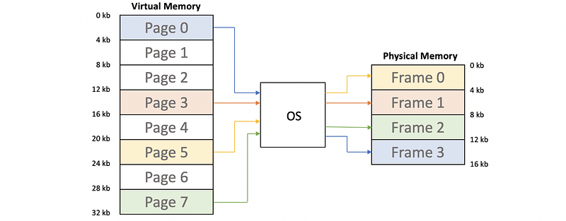
(3) Pages Vs. Page Frames

The virtual address space is subdivided into fixed-size segments that we call pages. The physical memory is divided into page frames of the same size. The role of the OS is to map pages from the virtual memory into page frames of the physical memory.

(4) Segment-Based Memory Management

Paging is not the only way to decouple the virtual and the physical memory. Another approach is segmentation so which would be a segment-based memory management approach.

With segmentation, the allocation process doesn’t use fixed-sized pages. Instead, it uses more flexibly sized segments that can be mapped to some regions in physical memory. Arbitration of accesses in order to either translate or validate the appropriate access uses segment registers that are typically supported on modern hardware.

However, paging is the dominant method used in the current OSs and we will mainly focus our discussion on page-based memory management in this section.

(5) Hardware Supports for Memory Management

The memory management unit (aka. MMU) in the hardware can be used to support memory management.

• First, the CPU issues virtual addresses to the MMU
• Second, the MMU translates VAs into the corresponding PAs
• Or potentially, the MMU can generate a fault. The faults are an exception or a signal that is generated by the MMU that can indicate illegal access (e.g. access memory not allocated), inadequate permissions (e.g. no writing permissions), or non-existing pages (e.g. file not found in memory).

Since the memory address translation happens frequently, most MMUsd would integrate a small cache of virtual to physical (V2P) mappings and this is called the translation lookaside buffer (aka. TLB). The presence of TLB will boost the V2P translation because we don't need to translate by page tables.

Although the actual V2P translation is done by the hardware, the OS maintains data structures such as the page tables. Thus, the hardware implies,

• what type of memory management modes are supported
• what kinds of pages can there be

(6) Software Supports for Memory Management

There are other flexible aspects of memory management since they’re performed in software. For instance, the actual allocation determining which portions of the main memory will be used by which process, or the replacement policies that determine which portions of the state will be in main memory vs on disk.

We will focus our discussion on those software aspects of memory management since that’s more relevant from an OS’s perspective.

2. Page Tables

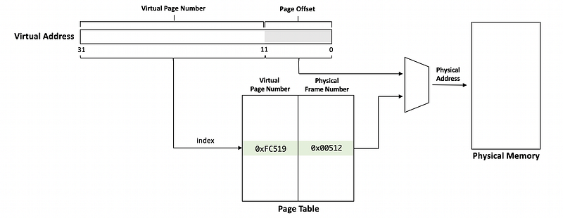
(1) Page Tables

In the page-based memory management system, the arbitration of the accesses is done by page tables. Page Tables are like a map that can be used to translate virtual memory addresses into physical memory addresses.

A virtual address consists of two parts, the virtual page number, and the page offset. The virtual page number is used as the index to the page table, and then it will be translated to a physical frame number based on the mappings in the page tables. The offset will be added to the frame number to create the physical address.

The physical memory for the virtual address space (or virtual address array) is only allocated when the process during its first initialization routine init_array(&array_addr). We refer to this as allocation on the first touch. The reason for this is that we want to make sure that physical memory is allocated only when it’s really needed because some of the virtual addresses are not going to be used by us.

The page table also maintains a valid bit (aka. present flag) that tells whether we have a corresponding physical memory in the memory. If the valid bit is set to 0, then the MMU can know that the page we request is not in the memory. So it will raise a fault.

Finally, the OS creates a page table for every process that it runs. That means that whenever a context switch is performed, the OS has to make sure that it switches to the page table of the new context switched process. We said that hardware assists with page table access by maintaining a register (e.g. CR3 for x86 system) that points to the active page table.

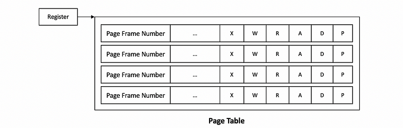
(2) Page Table Entries (PTE) Flags

Now, let’s focus on the page table and see how does its entry look like. We have known that the page table is used for mapping the virtual memory to the physical memory. What we don’t know is that the page table also stores the information for each of the pages for hardware and software interpretations. Thus, except for the page frame number (PFN), there are also many other useful flags in each entry. The most common flags are,

• Present flag (P): we have already discussed this flag as the valid bit and it is used to indicate whether the content is actually present in physical memory or not
• Dirty flag (D): this is used for file systems where files are cached in the memory, then we can use this bit to detect which file has been written to so that we can update the disk in the future
• Access flag (A): this can be used to track whether the page has been accessed for read or for write
• Protection Bits (R/W/X): the protection bits can be used to show the permission of the page (e.g. write-only, read-only, etc.)

(3) Page Table: An Example

Now, let’s see a real Pentium x86 page table entry,

its flags are,

• P: which is exactly the same as the present flag
• D: which is exactly the same as the dirty flag
• A: which is exactly the same as the access flag
• R/W: permission bit. 0 means read-only and 1 means read/write
• U/S: permission bit. 0 means user mode and 1 means supervisor mode only
• Other flags: for caching-related info (write-through/write-back, caching disabled, etc.)
• Unused bits: for future use

(4) Page Fault

The MMU uses the page table entries not only for the V2P translation but also relies on some bits of each entry to detect the validity of access. The page fault means that the MMU find out that the VA can not translate to PA. After that, the CPU will place an error code on the stack of the kernel and then it will generate a trap into the OS kernel. Then based on the error code, the kernel will call a page fault handler that determines what is the following actions need to be taken.

Key pieces of information in this error code will include whether or not the fault was caused because of,

• the non-existing page: need to load from the disk
• protection error: means there is a permission problem (i.e. SIGSEGV)

(5) Page Fault: An Example

On x86 platforms, the error code information is generated from some of the flags (e.g. PTE flags). The faulting address that is stored in a register CR2 is also needed during the page fault handler.

(6) Recall: Page Table Size

Now, let’s see how we can calculate the size of a page table. We will do the calculation for both the 32-bit system and the 64-bit system. Because we have only a 1-level page table, then this is called a flat page table. We have done this calculation in the following article and now we will do it again.

As we have known, the size of a flat page table can be calculated as,

Thus, suppose we have a 32-bit system, which means that each virtual address and each PTE have 32 bits. Thus, we can have 2³² virtual addresses and each address has a 1-byte storage. Suppose the page size is 4 KB (which is the most common value), then the page table size for this 32-bit system would be,

size_32 = 2^32B/4KB * (32/8)B = 4 MB

Also, for a 64-bit system, we can have,

size_64 = 2^64/4KB * (64/8)B = 32 PB

we can find out that for both the 32-bit system and the 64-bit system, the size of the page tables can be too large for us. Thus, it is not okay for us to have a flat page table in reality.

(7) Recall: Multi-level Page Tables

To have the same page table with a lower cost, we can consider using multi-level page tables. In a 2-level page table model, the outer page table (aka. top page table) can be treated as the page table directory. The internal page table has proper page table components like PFN and the flags, and they will be held only for those valid physical memory regions.

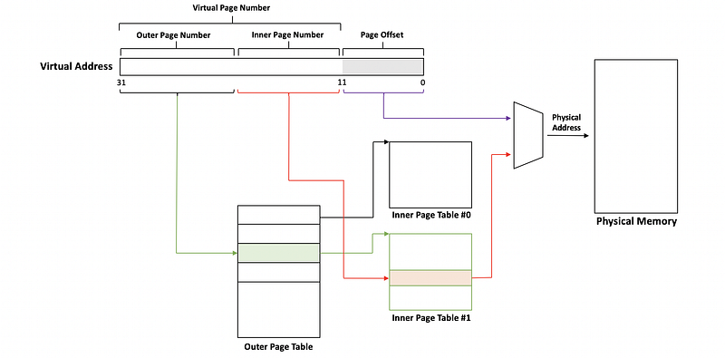
The size of the page tables will be significantly reduced because we will not maintain the inner page tables that are never accessed because the corresponding pages in the virtual address space can never be never used.

This technique is particularly important in 64-bit architectures because not only for the larger page table requirements but also for more sparse in the virtual address space. With more sparse, it will have larger gaps in the virtual address space region. Therefore, with 4-level addressing, we may end up saving the entire page table directories as a result of certain gaps in the virtual address space.

The problem with the MLPT is that the page tables are always stored in the memory and we need more access to the memory if we have more levels of the page tables. Thus, the overall performance will be slow down. We can deal with this by using the page table cache called the translation lookaside buffer (TLB).

(8) Recall: Translation Lookaside Buffer (TLB)

On most architectures, MMU integrates a hardware cache that’s dedicated to caching address translations. This cache is called the translation lookaside buffer (TLB).

On each address translation, first, the TLB cache is quickly referenced and if the resulting address can be generated from the TLB contents, then we have a TLB hit and we can bypass all of the other required memory accesses to perform the translation.

Or if we have a TLB miss, this means that the address isn’t present in the TLB cache. Then we have to perform all of the address translation steps by accessing the page tables from memory.

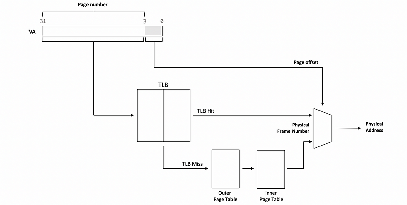
In addition to the proper address translation, the TLB entries will contain all of the necessary protection and validity bits to verify that the access is correct or, if necessary, to generate a fault.

As a result, it turns out that even a small number of entries in the TLB can result in a high TLB hit rate and this is because we have typically a high temporal locality and spatial locality in the memory references.

For instance, for each core on the recent x86 Core i7 platform, there would be,

• 64-entry TLB for data
• 128-entry TLB for instructions

And there is also a shared TLB for all the cores which has 512 entries.

(9) Inverted Page Tables (IPT)

Another completely different way to deal with the V2P translation is to create so-called inverted page tables. Instead of each entry in the page table corresponds to a virtual page number, each entry in the page table will be assigned a physical frame number. This is because we can at most have 10 GB physical memories, while we can have an O(PB) virtual memory address space. Thus, a mapping rule based on the physical frame number will make the page table much smaller.

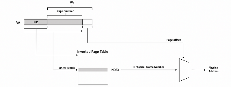
To find the translation, the inverted page table is searched based on the process ID (aka. PID) and the virtual page number. When the appropriate page number is found in the page table, the index will denote the physical frame number of the memory location that’s indexed by this logical address.

Since the physical memory can be arbitrarily assigned to different processes, the table isn’t ordered. So the problem is that we have to perform a linear search in order to find the corresponding PID and page number in the inverted page table. You can imagine that the linear search is really slow and it impacts our performance in general, even though TLB handles most of the V2P translations.

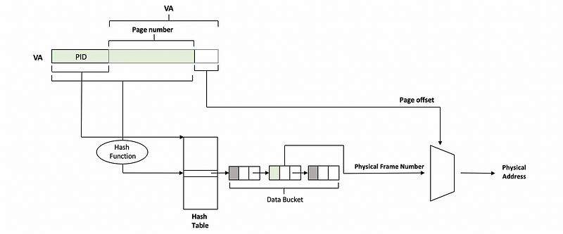
(10) Hashing Inverted Page Tables

We have discussed that it is such a serious problem for us if we need to do a linear search. To improve the performance, we can consider using the hash table. Instead of linear searching the whole inverted page table, we will replace it with a hash table with linked lists correspond to each entry of this table. We will conduct hashing on the PID and the page number and then work out a value to indexing the hash table. From this table, we can get a pointer that points to the data bucket. Then we will search the PID and the page number in this bucket and if we find it, we will get the frame number associated with this element in the bucket.

(11) Choosing Page Size

There are some benefits to have a larger page size, for example, we can have

• fewer page table entries
• smaller page tables
• more TLB hits
• etc.

However, there can also be some internal fragmentation and the memory can be wasted because of that. Thus, we will commonly have a 4KB page size.

3. Segmentation

(1) An Introduction to Segmentation

Instead of pages, the V2P translation can also be performed using segments. In this section, we are going to briefly introduce this approach. Actually, the process is referred to as segmentation.

(2) Segmentation Features

With segments, the address space is divided into components of arbitrary granularity of arbitrary size. Typically, the different segments will correspond to some logically meaningful components of the address space like

• the code
• the heap
• the data
• etc

A segment could be represented with a contiguous portion of physical memory. In that case, the segment would be defined with its base address and its limit registers which implies also the segment size.

(3) Segmentation Implementation

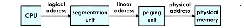
A virtual address in the segmented memory mode includes a segment descriptor and an offset. The segment descriptor is used in combination with the descriptor table to produce information regarding the physical address of the segment.

The result of the segmentation is called a linear address instead of a physical address, so segmentation must be used with paging.

Briefly, this is equivalent for us to have,

(4) Segmentation Example

If we look at the intel platforms, the x86 platforms,

• on 32-bit hardware: both segmentation and paging are supported. Linux allows up to 8000 segments to be available per process and another 8000 global segments.
• on 64 bit hardware: even though segmentation and paging are supported for backward compatibility, the default mode is to just use paging

4. Memory Allocation

(1) The Definition of Memory Allocation

We have discussed how to do a V2P translation, but what we didn’t explain was how the OS allocates the memory. This is the job of the memory allocation mechanisms that are part of the memory management subsystem of an OS, which answers what are the physical addresses that will correspond to a specific virtual address. This mapping is established by the memory allocator.

(2) Kernel-Level and User-Level Memory Allocator

Memory allocators can exist at both the kernel level and the user level.

Kernel-level memory allocators are responsible for allocating memory regions such as,

• kernel pages for various components of the kernel state
• static state for the processes when they’re created (e.g. for code, stack, or initialize data)
• keep track of the free memory that’s available in the system

User-level memory allocators are used for dynamic process states like,

• the heaps (i.e. the dynamic process state)
• basic interface: malloc / free

Once a kernel allocates some memory to a malloc call, the kernel is no longer involved in the management of that space. That memory will at that point be used by whatever user-level allocator is being used, and there are a number of options out there right now that have certain different trade-offs. We will list some of them here but we are not going to discuss the detailed usage of them. These options are,

• dlmalloc
• jemalloc
• hoard
• tcmalloc

(3) External Fragmentation

External fragmentation can happen if we must allocate a range of coutinous memory. Let’s see an example. Suppose we have 16 frames in the physical memory and we then conduct the following code,

L1: alloc(2), alloc(4), alloc(4), alloc(4)
L2: free(2)
L3: alloc(4)

If the physical frames are allocated in order from the beginning of the physical memory, then after L1 and L2, we will have,

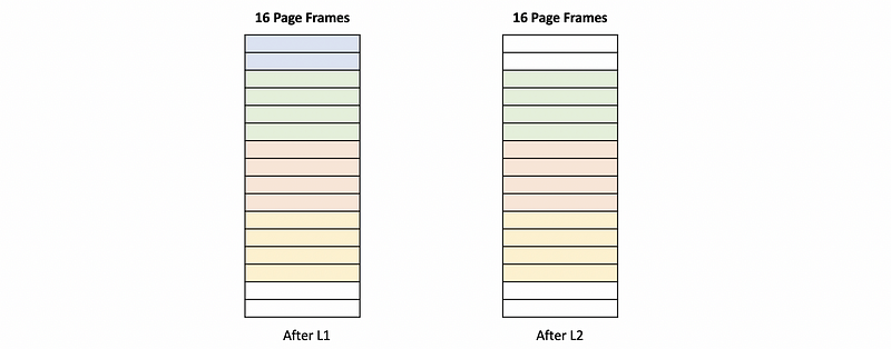
We can find out that even though we have 4 free frames, we can not allocate these 4 frames at a time because these frames are not continuous. Thus, the memory allocator can not meet the requirement for L3. One downside of the external fragmentation is that we will have holes of free memory that are not contiguous. Thus, even we have enough space for allocation, the memory allocator can not conduct that.

(4) External Fragmentation: Solution

Let’s consider an alternative, in which the memory allocator probably knows something about the requests that are coming. So in the 2nd case, when the 2nd request for allocating 4 pages comes, the memory allocator isn’t allocating it immediately after the first allocation, but instead, it’s leaving some gap.

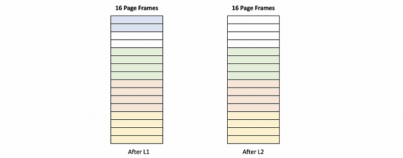
Now when the free request comes in, these 2 first pages are freed. The system again has 4 free pages and they’re consecutive. Therefore this next request for 4 free pages can actually be satisfied in the system.

What we see in this example, is that when these pages are freed there was an opportunity for the allocator to coalesce or to aggregate these adjacent areas of free pages into one larger free area in order to satisfy the need of future allocate requirements.

(5) Linux Memory Allocators #1: Buddy Memory Allocator

Basically, the Linux OS has two kinds of memory allocators that can deal with external fragmentation problems. These memory allocators are called the buddy allocator and the slab allocator. We will first have a look at the buddy allocator.

The buddy allocator starts with some consecutive memory region that’s free that’s of a size of 2ⁿ. Whenever a request comes in, the allocator will subdivide this large request into smaller chunks such that every one of them is also a 2ⁿ. Then it will continue subdividing until it finds the smallest chunk that’s with a size of a power of 2ⁿ that can satisfy the request.

Let’s see an example. Suppose we want to allocate 8 frames and we have a 64-frame physical space. To have a larger continuous memory region, we will divide the memory region and allocate memory from the bottom of the physical space.

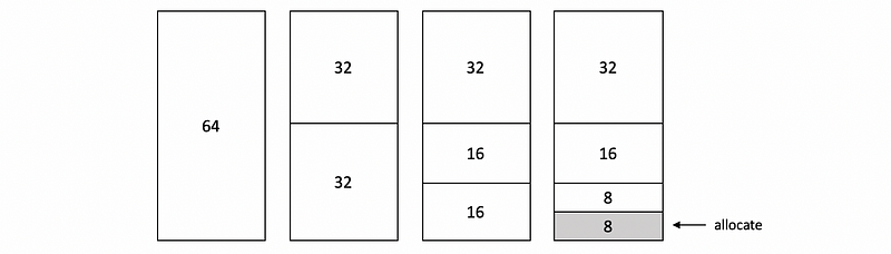
The reason why these areas are 2ⁿ is that the addresses of each of the buddies differ by only 1 bit, which makes it easier to perform the necessary checks when combining or splitting chunks.

(6) Buddy Memory Allocator Evaluation

The benefit of the buddy algorithm is that the aggregation of the free areas can be performed really well and really fast.

However, the fact that allocations using the buddy algorithm have to be made in the granularity of 2ⁿ means that there will be some internal fragmentation using the buddy allocator. This is particularly a problem because there are a lot of data structures that are common in the Linux kernel that are not of a size that’s close to 2ⁿ. This is why we have the slab allocator.

(7) Linux Memory Allocators #2: Slub Memory Allocator

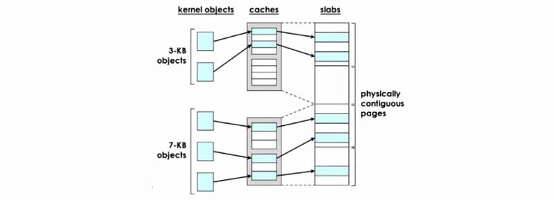
To fix the internal fragmentation issues, Linux also uses the slab allocator in the kernel. The allocator builds custom object caches on top of slabs, and the slabs themselves represent contiguously allocated physical memory.

When the kernel starts it will pre-create caches for the different object types. For instance, it will have a cache for task_struct or for the directory entry objects, then when an allocation comes for a particular object type then it will go straight to the cache and it will use one of the elements in this cache. If none of the entries is available, then the kernel will create another slab and it will pre-allocate an additional portion of contiguous physical memory to be managed by the slab allocator.

The benefits of the slab allocator are,

• it avoids internal fragmentation
• external fragmentation is not really an issue

5. Demand Paging

(8) The Definition of Demand Paging

Because the virtual address space can be much larger than the physical memory, so sometimes we have to store some information on the secondary storage (e.g. disk) and when we need them, we can load them back from the secondary storage. This is called demand paging. The procedure of demand paging is illustrated in the following diagram.

Finally, we need to have 2 final insights,

• First, the original physical address of this page will very likely be different from the physical address after this demand paging process was over
• Second, if for whatever reason we require a page to be constantly present in memory or if we require it to maintain this same physical address during its lifetime, then we will have to pin the page. So at that point, we basically disable the swapping. This is for instance useful when the CPU is interacting with devices that support direct memory access (DMA).

(9) Page Replacement: When to Swap Out?

There are two remaining problems of the demand paging,

• When should the pages be swapped out from the physical memory onto the disk?
• Which pages should be swapped out?

Let’s first answer the first problem. Periodically, when the amount of occupied memory reaches a particular threshold, the OS will run some page(out) daemon that will look for pages that can be freed. So in the following two cases, we are going to have some pages swapped out,

• when memory usage is above the threshold, this is called high watermark
• when CPU usage is below the threshold, this is called low watermark

(10) Page Replacement: Which to Swap Out?

To answer the second question, one obvious answer would be that the pages that will not be used in the future are the ones that should be swapped out. The problem is how do we know which pages will vs won’t be used in the future? The answer is that we have to make some predictions regarding the page usage by some historic information.

One common algorithm is called the least recently used (LRU) policy, which will remove the page that hasn’t been accessed for a long time. This can rely on the access bit.

Another case is that when the page doesn’t need to be written out, we can swap them out with no disk written overheads. This can rely on the dirty bit.

6. Hardware Supported Techniques

(1) Copy-On-Write (COW)

Let’s see what happens during process creation. When we need to create a new process, we need to recreate the entire parent process by copying its entire address space. However, because many of the pages don’t change, we don’t need to keep multiple copies.

In order to avoid unnecessary copying, the newly created process will be mapped to the original page that had the original address space content. If the contents of this page are read-only, then we’re going to save both the memory and time for doing this copy.

However, if a write request is issued for this memory area via either one of these virtual addresses, then the MMU would detect that the page is write protected and will generate a page fault. At that point, the OS will see what is the reason for this page fault, will create the actual copy.

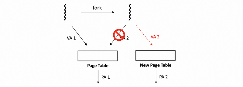
We call this mechanism copy-on-write because the copy cost will only be paid when we need to perform a write operation.

(2) Checkpointing

Checkpointing is a technique that’s used as part of the failure and recovery management that the OS supports. The idea behind checkpointing is to periodically save the entire process state. The failure may be unavoidable, however, with checkpointing the process doesn’t have to be restarted from the beginning. It can be restarted from the nearest checkpoint point and so the recovery will be much faster.

(3) Checkpointing Implementation

A simple approach to checkpointing would be to pause the execution of the process and copy its entire state.

A better approach will take advantage of the hardware support for memory management. Using the hardware support, we can write-protect the entire address space of the process and try to copy everything at once. However since the process will continue executing, it will continue dirtying pages. So then we can track the dirtied pages again using MMU and we will copy only the difference, which will allow us to provide for an incremental checkpoint.

(3) Rewind Replay

Debugging relies often on a technique called rewind replay. Rewind means that we will restart the execution of the same process from some earlier point. We can gradually go back to older and older checkpoints until we find the error.

(4) Migration

With migration, it’s like we checkpoint the process to another machine and then we restart it on the other machine, then this process will continue its execution. This is useful in scenarios such as disaster recovery and consolidation.