Probability and Statistics 1 | Basic definitions, 3 Axioms and 7 Theorems of Probability
Probability and Statistics 1 | Basic definitions, 3 Axioms and 7 Theorems of Probability

- Random Experiment
(1) Functions are not Random Experiments
A function is that with a given x, we can do calculations and f(x) could be known. For example, with the function f(x) = x², x is the input and x² si the output. So this is not a random experiment.
(2) Definition of Random Experiment
A random experiment is a process or action whose outcome is not determined. For example, like stochastic.
(3) Examples of Random Experiment
If we are rolling a die or dealing outa a deck of cards, these manners we are conducting are random. Other examples like the weather at 12 noon on 5/30/2060 at San Francisco.
2. Sample Space
(1) Definition of the Sample Space
The set of all possible outcomes of a random experiment is called the sample space. We typically denote the sample space by S or Ω.
(2) Definition of the Outcomes
We call the elements of S (or Ω) outcomes (or atoms or singletons). They are denoted by s or ω.
(3) The relation between Sample Space and Outcomes
If we flip a coin three times (order matters), we can have the possible sample space like the following graphic.

(4) Definition of the Events
An event (typically denoted with capital letters like A and B) is (kind of) any subset of S.
- we can write things like A⊆S, B⊆S, or A∩B⊆S
- all set operations (i.e. ∩, ∪, ∈) can be used with events
(5) ℙ Notation
You may have seen notations like ℙ(A) or ℙ(B) = ℙ(x ≥ 5) [Note: this has the same meaning of B = {s∈S |x(s) ≥ 5}.] So what makes ℙ a probability measure on S? The answer is that this is the axioms of Kolmogorov.
(6) Kolmogorov Framework
Let S be a sample space and let ℙ become a function ℙ = P(S) → ℝ, where P(S) means the set of all subsets of S or briefly the power set of S. We say the ℙ is a probability measure and (S, ℙ) is a probability space if:
- Axiom #1: ℙ(A) ≥ 0 for any event A⊆S (Non-negativity)
- Axiom #2: ℙ(S) = 1 (Unity)
- Axiom #3: If A1, A2, A3, … is a sequence of mutually exclusive events, then (countable additivity)

(7) Definition of Mutually Exclusive
Events A and B from S are mutually exclusive if A ∩ B = ∅. So, if A1, A2, … is a sequence of mutually exclusive events, then ∀i, ∀j, Ai ∩ Aj = ∅.
3. Theorems Related to ℙ
(1) Theorem #1: ℙ(∅) = 0
Proof:
Assume that I have a probability space (S, ℙ), let A1 = ∅, A2 = ∅, A3 = ∅, …
Because ∅∩∅ = ∅, {Ai|i=1→∞} is mutually exclusive
⇒ can apply axiom #3
⇒ we have
Note that,

But also, by Axiom #1, ℙ(∅)≥0,
So for case #1, if ℙ(∅)>0:
Suppose that ℙ(∅) = c > 0
But then,

Since 0<c<1<∞, this is a contradiction.
So, in conclusion, ℙ(∅)= 0.
(2) Theorem #2: (finite additivity)
If A1, A2, A3, … is a finite sequence of mutually exclusive events, then

Proof:
Construct an infinite sequence of events as follows:
B1 = A1, B2 = A2, B3 = A3, …, Bn = An, Bn+1=∅, Bn+2 = ∅, …
Obviously that, for ∀i, ∀j, Bi ∩ Bj = ∅
So the sequence of {Bi | i=1 → n} is mutually exclusive
⇒ can apply axiom #3
So that,

Meanwhile,

Therefore,

Which is also the same as,
(3) Theorem #3: If A ⊆ B, then ℙ(A) ≤ ℙ(B)
Proof:
[NOTE #1: First use of disjunctification, which is to write a set as the union of mutually exclusive sets. ]
[NOTE #2: If A ⊆ B, then B = A ∪ (B ~ A). The notation of B ~ A equals B ∩ ~A, and ~A is the complementary set of set A. This is shown by the following Venn diagram. ]
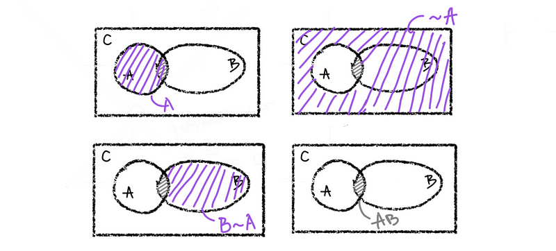
Proof of NOTE #2:
Based on the Venn diagram,
B~A = B ∩ ~ A = B - B ∩ A
if A ⊆ B, B ∩ A = A
so, B~A = B - A
therefore, A ∪ (B ~ A) = A ∪ (B - A) = B
Proof of this theorem:
ℙ(B) = ℙ(A ∪ (B ~ A)) = ℙ(A) + ℙ(B ~ A)
ℙ(B ~ A) = ℙ(B - B ∩ A), and with A ⊆ B, then, B ∩ A = A
so, ℙ(B ~ A) = ℙ(B - A) = ℙ(B) - ℙ(A)
Because A ⊆ B, by Axiom #1, we have, ℙ(B) - ℙ(A) ≥ 0
So that, ℙ(B) ≥ ℙ(A)
Aside: If we have ℙ(A) = 0, we cannot conclude that A = ∅
Exception: If v~Unif(0,1), then ℙ(U=1/π) = 0, but {1/π} ≠ ∅
(4) Theorem #4: ℙ(A) = 1 - ℙ(~A) (Complementarity)
Proof:
By Axiom #2, we can have ℙ(S) = 1
Obviously, ℙ(S) = ℙ(A∪(~A)) = ℙ(A) + ℙ(~A) = 1
⇒ ℙ(A) = 1 — ℙ(~A)
(5) Theorem #5: For any events A ⊆ S, 0 ≤ ℙ(A) ≤ 1
Proof:
Recall, ∅ ⊆ A ⊆ S, by Theorem #3, ℙ(S) ≥ ℙ(A) ≥ ℙ(∅)
by Theorem #1, ℙ(A) ≥ ℙ(∅) = 0
by Axiom #2, ℙ(A) ≤ ℙ(S) = 1
(6) Theorem #6: ℙ(A ∪ B) = ℙ(A) + ℙ(B) - ℙ(A ∩ B ) (HIGH SCHOOL THEOREM)
⇒ ℙ(A ∪ B) = ℙ(A ∪ (B~(A ∩ B)))
⇒ ℙ(A ∪ B) = ℙ(A) + ℙ(B~(A ∩ B))
⇒ ℙ(A ∪ B) = ℙ(A) + ℙ(B) - ℙ(A ∩ B)
⇒ ℙ(A ∪ B) = ℙ(A) + ℙ(B) - ℙ(A ∩ B)
Note: this theorem has a generalization called the inclusion-exclusion principle that tells you how to compute probabilities of unions of more than two sets. For example:
ℙ(A ∪ B ∪ C) = ℙ(A) + ℙ(B) + ℙ(C) - ℙ(A ∩ B) - ℙ(B ∩ C) - ℙ(A ∩ C)
(7) Theorem #7: Let S be a discrete and finite sample space, i.e.

If the members of S are equally likely (which means two events A and B have the same probability, ℙ(A) = ℙ(B)), then ℙ({Si}) = 1/n, when n =|S|(which means the number of elements in S)
Proof:
by Axiom #2: 1 = ℙ(S)
then by theorem #2,

then,

therefore, ℙ({Si}) = 1/n.