Probability and Statistics 2 | Conditional Probability, Independent Events, The Law of Total…

Probability and Statistics 2 | Conditional Probability, Independent Events, The Law of Total Probability, and Bayes Theorem

1. Conditional Probability

In the previous part, we have already introduced the 3 axioms and the 7 facts of the probability measures. So how could we create new probability measures from the old ones? One answer (not the only answer) to this question is the conditional probability.

(1) The Mathematical Definition of Conditional Probability

Suppose that (S, ℙ) is a probability space. Let A and B be events such that ℙ(B) > 0. Suppose that we propose a new probability measure Q and define,

But now, we are not sure about whether Q is a probability measure that in its own right, so we have to check the three axioms.

(2) Conditional Probability on Axiom #1

Proof:

Because ℙ is a probability measure, so we have ℙ(A∩B) ≥ 0

Because we have the assumption in the definition that ℙ(B) > 0,

So, check

(3) Conditional Probability on Axiom #2

For B ⊆ S, so that S ∩ B = B.

So, check

(4) Conditional Probability on Axiom #3

Let A1, A2, … be a sequence of mutually exclusive events. Check,

This means that all theorems from the last part hold for the probability measure Q.

(5) The Conceptual Definition of Condition Probabilities

We want to “assume” that B occurs and then recompute then probabilities (i.e. of A) based on the assumption that B occurs. And we often write like,

Here is an example,

2. Independent Events

(1) The Definition of the Independent Events

If event A and B are independent, so

(2) The Theorem of Independent Events

We can also have the conclusion that if A and B are independent

Proof:

By definition of the conditional probability ⇒ ℙ(A ∩ B) = ℙ(A|B)ℙ(B)

Given that A and B are independent, by definition ⇒ ℙ(A|B) = ℙ(A)

Therefore, ℙ(A ∩ B) = ℙ(A)ℙ(B)

(3) Positively and Negatively Correlated

If events A and B are not independent, we can say that they are correlated with each other.

• if A and B are positively correlated ⇒ ℙ(A|B) > ℙ(A)
• if A and B are negatively correlated ⇒ ℙ(A|B) < ℙ(A)

3. The Law of Total Probability

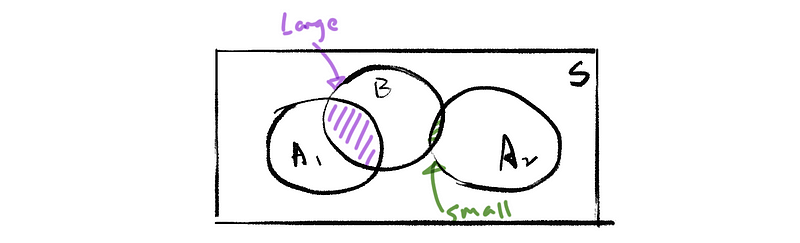
(1) Partition Sequence (aka. Decomposition Sequence or Covering Sequence)

Suppose that we have a sequence of events B1, …, Bn (finite) or B1, B2, … (infinite) on a probability space (S, ℙ) and it satisfies:

• Mutually Exclusive

• Covering Property: it covers the whole set

• Non-triviality

We call such a sequence a partition or decomposition or covering sequence of S.

(2) The Law of Total Probability

If B1, B2, …, Bn is a partition sequence of S, and A is any event, then,

Proof:

By definition of the conditional probability,

By finite theorem,

By covering property argument (or by element-wise proof, which means to separate the notation and calculate element by element), we could have,

Also, it is quite obvious that the sequence {A ∩ Bi} is mutually exclusive. Because we have already known that the sequence {Bi} is mutually exclusive by definition, so we can obviously understand why the sequence {A ∩ Bi} is mutually exclusive.

(3) The Law of Total Probability: An Example

Calculate the probability of the widget fails.

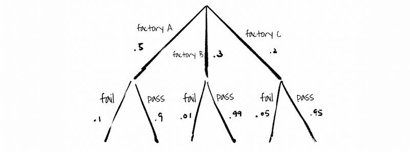
Solution:

By the law of total probability, A ∩ B ∩ C = S, then

ℙ(widget fails) = ℙ(fail|A)ℙ(A) + ℙ(fail|B)ℙ(B) + ℙ(fail|C)ℙ(C)

ℙ(widget fails) = .063

4. Bayes Theorem

(1) Bayes Theorem

Suppose that (S, ℙ) is a probability space and B1, B2, …, Bn, … is a partition of S.

Proof:

First of all, based on the definition of the conditional probability,

Then, by infinite activity,

With the definition of conditional probability,

(2) Bayes Theorem: An Example

Given that a widget has failed, what is the probability that it came from factory C? Suppose that event B1 = factory A, B2 = factory B, B3 = factory C, D = widget failure.

Solution:

By Bayes theorem

ℙ(B3|D) = ℙ(D|B3)ℙ(B3)/[ℙ(D|B1)ℙ(B1)+ℙ(D|B2)ℙ(B2)+ℙ(D|B3)ℙ(B3)]

ℙ(B3|D) = .05*.2/.063 = .16