Probability and Statistics 3 | Random Experiment, Probability Mass Function, Probability Density…
Probability and Statistics 3 | Random Experiment, Probability Mass Function, Probability Density Function, and Cumulative Density Function

- Random Experiment
(1) The Definition of Random Experiment and Outcome
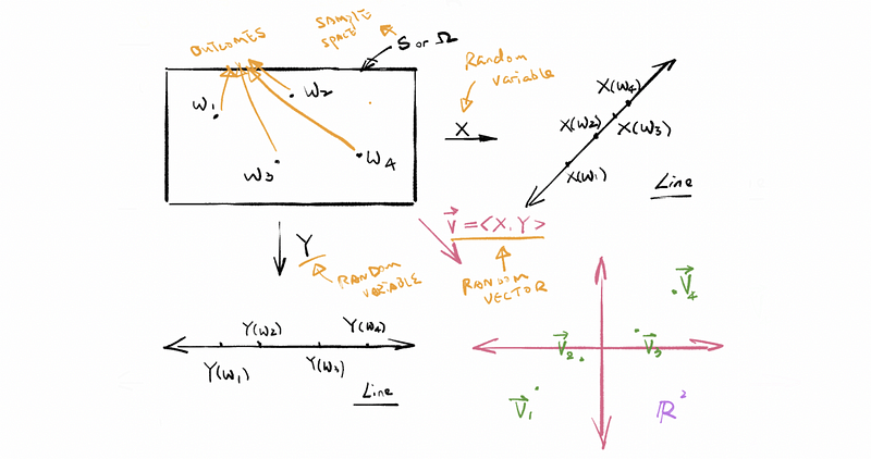
A random experiment is any activity, process, or action that produces a non-deterministic (i.e. Stochastic) outcome. An outcome is a result of a random experiment. The set of all possible outcomes is called the sample space.
(2) The Definition of Random Variable (aka. r.m.)
A random variable is a function from {the set of all possible outcomes from some random experiment} to the real number line. The notations of the random variable are capitalized letters, for example, X, Y.
For example, choose 25 folks inside the United States at random (and without replacement). Call a particular outcome w1.
- X(w1) = averages the heights (in centimeters) of the folks associated with w1.
- Y(w1) = max weight (in kilograms) of the folks associated with w1.
(3) The Definition of Random Vector
A random vector is a function from {the set of all possible outcomes from some random experiment} to real space, or ℝⁿ, or n-dimensional real space. The notations of the random variable are capitalized bold letters, for example, X and Y. For example,
- X(w1) = <X(w1), Y(w1)>
- X(w1) = <160, 67>
- X(w2) = <145, 72>
- X(w3) = <164, 80>
2. Types of Data or Random Variables
(1) Binary (aka. Bernoulli): the data are either zeros or ones or can be mapped to such. For example:
- bio gender
- {switch is off, switch is on} ← mutually exclusive
(2) Categorical: the data that maps into mutually exclusive categories. For example,
- Integrated Postsecondary Education Data System
- Race / Ethnicity
- {A+, A, A-, B+, B, B-, C+, C, C-, F}
(3) Ordinal: This is categorical data that admits a natural ordering. For example,
- grades
- quartiles
- {1st place, 2nd place, 3rd place}
(4) Continuous (aka. Quantitative or Numerical): The data that maps naturally onto the real number line. For example,
- the stock price
- temperatures
- heights
3. Probability Mass Function (PMF)
(1) Support Set
The support set A of some random variable X is all those real values that can be or might be, naturally obtained by X. While x is an element (one of the real value of the random variable X) of the support set A. For example,
- ℝ* is the support set for a random variable that measures the height.
- Roll a die and look at the top face. The support set A = {1, 2, 3, 4, 5, 6}, and x could be 1 or 2 or 3 or 4 or 5 or 6.
(2) The Definition of the Probability Mass Function
The probability mass function is a function p(x) → ℝ, where A is the support set of an associated random variable X and p is called the probability mass, satisfies the following two properties,
- Axiom #1(Non-negativity): If x ∈ A, p(x) = ℙ(X = x) = ℙ({ w∈Ω | X(w) = x }) ≥ 0
- Axiom #2 (Unity): for x∈A,

Note that we haven’t got an axiom #3 here. This is partly because the form of the countable additivity (or Axiom #3) is quite simple and obvious to p(x) and we can directly compute that from Axiom #1. The proof is,
Proof:
Suppose that we have infinite random variables X1, X2, X3, … which are mutually exclusive. Given Xi, ∀ real values xi of the support set Ai would satisfy,

So, we can then have,

So it would be possible if we write,

Well, this notation is not commonly used and just a simplified version of proving Axiom #3. It may have some contradiction in the notation because when we talk about p(x), we usually talk about one SINGLE random variable X. But in the proof before, we obtained these “xi”s from different random variable Xi. So that may be confused, and I want to clarify that this is not a rigorous proof.
(3) The Notation of Probability Mass Function
In the previous proof, we can find out that the PMF p(x) is highly related to the random variable X. So in order to stress the dependence of probability mass p on X, we often write notations like,

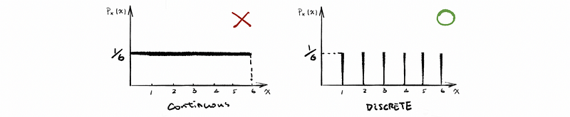
(4) Probability Mass Function: Die Rolling Example
In this case, we have six discrete outcomes as Ω = {“top face = 1”, “top face = 2”, “top face = 3”, “top face = 4”, “top face = 5”, “top face = 6”}. For each of the outcome wi ∈Ω, the random variable function X(wi) changes different outcomes into discrete numbers. For example, X(“top face = 5”) = 5.
Therefore, as we have told that the support set A of X equals {1, 2, 3, 4, 5, 6}, and each of the elements in this set is reckoned to be the real value x. So because all the real values, in this case, are equally likely, then we can have the probability mass p as,

4. Probability Density Function (PDF)
(1) The Definition of Probability Density Function
A probability density function (PDF) is a function f from the real number to the real number line. For example, f: ℝ (or we could say the support set) → ℝ. It has two properties:
- Non-negative: ∀ x ∈ℝ, f(x) ≥ 0, because a negative one will violate Axiom #1
- Unity:

Note that it is not a requirement on f that 0 ≤ f(x) ≤ 1, ∀ x ∈ℝ. However, it is a requirement for p(x) that 0 ≤ p(x) ≤ 1. And also, because we want to stress the dependence of probability mass f on X, we write notations as,

(2) Probability Density Function: An Example
The PDF of a normal variable is given by,

We denote such a situation, i.e., where X is normal by X ~ N(μ, σ²). If we take σ → ∞, f becomes large about μ ⇒ f ≰ 1. Especially, if X ~ N(0, 1), it is called standard normal.
(3) The Proof of Whether a Proper PMF or a Proper PDF
We use Infinite Series to prove a proper PMF and we use Integration to prove a proper PDF. For example:
- Example 1. Is this a proper PMF?

Clearly that p(x) ≥ 0, so we have to prove unity. Then,

- Example 2. Is this a proper PDF?

Clearly that f(x) ≥ 0, so we have to prove unity. Then,

5. Cumulative Distribution Function (CDF)
(1) The Definition of Cumulative Density Function
The cumulative distribution function is another way of encoding the information in the PDF or PMF. It is typically denoted F or Fx(t).

(2) Cumulative Density Function: A Discrete Example
For example,


For a discrete random variable X,


(3) Cumulative Density Function: A Continuous Example
For example,


For a continuous random variable X,


(4) Probabilities of Cumulative Density Functions: Every function F is a CDF if,
- F is non-decreasing, i.e., if s ≤ t, F(s) ≤ F(t)
- As t → -∞, F(t) → 0, which is also,

- As t → +∞, F(t) → 1, which is also,

- F must be a right-continuous function, i.e., ∀ s∈ℝ,

6. Method of Inverse Transformations
(1) Result of Borel
If you can write down a proper PDF, PMF, or CDF, then there exists a random variable X on some probability space (S, ℙ) such that the PDF, PMF, or CDF associated with your X will be exactly that you wrote down.
(2) Uniformly Distribute
If X ~ Unif [a, b], we say that X is uniformly distributed over the interval [a, b]. i.e. it has PDF of,


then the CDF must be,

(3) Method of Inverse Transformations
Three things to get started:
- You need a random variable X for which you want to simulate a realization (or outcome)
- You need an explicit (or even implicit) inverse of the CDF for X, i.e., an inverse Fx‾ ¹
- You need the ability to simulate uniform random numbers on [0, 1]
Algorithm:
- Simulate a U ~ Unif(0, 1)
- Construct,

- Store it and loop back to the first step as many times as you need realizations.