Probability and Statistics 5 | Joint Probability, Independence of Random Variables, and Condition…

Series: Probability and Statistics

Probability and Statistics 5 | Joint Probability, Independence of Random Variables, and Condition Probability in Bivariate Context

Joint Probability

If X is a random variable with density fx(x) and Y is a random variable with density fY(y), how would we describe the joint behavior of the tuple (X, Y) at the same time? The answer is joint PDFs (density functions) and joint CDFs.

(1) The Definition of the Joint Probability Density Functions (2 r.v.)

A bivariate PDF is a function f: ℝ² → ℝ satisfying the following two properties:

Non-negativity

Unity

(2) The Definition of the Joint Probability Density Functions (n r.v.)

If X1, …, Xn are random variables with densities fX1(x1), fX2(x2), …, fXn(xn), their joint density is given by some function f: ℝⁿ→ ℝ with,

Non-negativity

Unity

(3) The Definition of the Bivariate Cumulative Distribution Function (2 r.v.)

Suppose that X ~ fX and Y ~ fY, the bivariate cumulative distribution function CDF of (X, Y) is defined as:

Note that the bivariate cumulative distribution function has the following 6 facts:

Fact #1

Fact #2

Fact #3: The function F must be non-decreasing.
Fact #4: The function F must be right-continuous.
Fact #5

Fact #6

(4) The Definition of the Multivariate Cumulative Distribution Function (n r.v.)

Suppose that Xi ~ fi = fxi, for i = 1, 2, …, n. The joint CDF of (X1, X2, …, Xn ) is a function F: ℝⁿ→ ℝ, defined as,

It is important to know that the multivariate CDF inherits properties analogous to the bivariate CDF, so we do not have to state again here but it is crucial to keep these properties in mind. For example,

2. Independent Random Variables

(1) Recall: Independence of Two Variables

What does the independence of random variables look like in light of those definitions? Now, let’s recall that A and B are independent events, that then, we have,

It is not a proper way to assign the event as the capitalized letter X and Y because it is usually unclear about the notation. For example,

this is not a good way to define independent variables because it would cause some ambiguous here. For the reason that X and Y are usually used to represent the random variables and here what we want to define is to treat X and Y as the event sets. So there has been inconsistency in our notation of X and Y, so it is definitely not a good idea to write things like that!

Suppose we have a demand to link the event set A with the random variable X (the conditions of r.v. X over outcomes is treated as out event set A), we can define the event set A as,

So now we have a method to link the conditional random variable X with set A and it is not random any more if we write things like,

therefore, if we also define that,

We can then apply the definition of independence to this specific case as,

(2) Formal Definition of Independent Random Variables

If, for every interval [a, b]∈ℝ and [c, d]∈ℝ, if we have

or we can also write as,

then, X and Y are independent random variables. An analogous definition holds in a multivariate context.

(3) Factorization Property of CDF: A Direct Consequence by Independent Random Variables

Choose that [a, b] ∈ (-∞, s] and [c, d] ∈ (-∞, t], if X and Y are independent, then,

which is also,

This is called the factorization property of CDFs under independence.

(4) Recall: the Relationship between the Density Function and CDF

If X is a random variable, let its density be fX(x) and Its CDF be FX(t), by definition, If X is continuous, then

Based on this fact, we can also derive the conclusion that,

Proof:

(5) Factorization Property of Densities (PDF)

So what happens in higher dimensions, say 2 dimensions? Let’s suppose that the random variable X and Y are independent. Based on our discovery of factorization property of CDF, that,

Then we calculate the partial derivative of F(s, t) on variable s, t and draw the conclusion that,

Proof:

then, we can have,

(6) Property of Expectation on Independent Random Variables

Let X and Y be independent random variables, then we have,

Proof:

By the definition of expectation, we can then have,

But since X is independent of Y, we have,

then,

then,

then,

then,

thus,

WARNING: The converse statement is not true, i.e., if X and Y are random variables such that,

it doesn’t necessarily mean that X⊥Y. (⊥ is the notation of “being independent of ”). For example, suppose random variable X ~ N(0, 1) and set Y = X². Clearly Y depends on X, which is also to say X and Y are not independent. But,

and,

so,

(7) Verify Independence for All Random Variables in a Sequence

Suppose we want to verify that X1, … , Xn is an independent sequence of random variables, does it suffice to check that Xi ⊥ Xj, ∀ i ≠ j ∈{1,2, …, n}?

In other words, if we want to check pairwise independence of a sequence to confirm the independence of the whole sequence, that works for me to check the exclusivities. Remember there was a lovely lazy track because of the special wired property of the empty set like if A ∩ B = ∅, then that ∩ anything else to be the empty set. So to establish visualized exclusivity of a sequence, we can just check out the pairs because the three-way intersection always includes the two-way intersection, which is the empty set. So by proving the mutual exclusivity for pairs, you then get anything else for free.

For example,

The bad news is no, and the property of exclusivities doesn’t happen here! If we check the independence of all pairs in a sequence, it won’t give us the conclusion that we can talk about it to the whole sequence freely. We have to, in theory, check all combinations of the Xi’s for the property that probabilities of intersections equal products of probabilities (or, for random variables. factorizations of joint densities).

Suppose we have events A, B, and C, and A and B are mutually exclusive, B and C are mutually exclusive, and then C and A are mutually exclusive, we can freely derive that,

But for events A, B, and C, and A and B are independent, B and C independent, and then C and A are independent, it is clear we could not derive that,

So if it doesn’t hold for events, it doesn’t hold for the random variables, so it doesn’t suffice to check merely in pairs, and we have to check all combinations!

(8) Geometrics: The Shape Independent Support Set

What does the shape of the support set of the tuple (X, Y) (for example) tell us about the possibility that X and Y are independent?

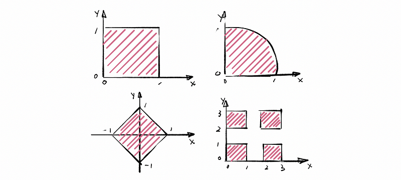
For the first graph (Square), given X = x∈[0, 1], we then have Y = y ∈[0, 1], because we cannot know any new information by given X = x as a condition, so random variables X and Y are possible to be independent.

For the second graph (Quarter circle), X = x∈[0, 1], when X = 1, we can derive that Y = 0. Because the value of random variable Y is going to depend on the random variable X, so the random variables X and Y are not independent.

For the third graph (Diamond), it is quite similar to the second graph that the value of random variable X could control the value of random variable Y, so the random variables X and Y are not independent.

For the last graph (Squares), it is quite similar to the first graph that the value of random variable X could not control the value of random variable Y, so the random variables X and Y are possible to be independent.

So in conclusion, the key requirement is that a necessary condition for the independence of random variables is that the support set of their joint density must be defined on a multi-dimensional rectangle, i.e. any number of intervals that are unioned, interested, complement, etc, and then crossed (in a cartesian) with another such set. Then, you may be able to define the random variables so that they are independent over the resulting support set. (We must also check the factorization condition of the random variables X and Y.)

3. Condition Probability in Bivariate Context

(1) Bivariate Condition Probability of Continuous Random Variables

Suppose that we have continuous random variables X and Y. Let f(x, y) be a joint PDF. The conditional density of X given Y = y is,

Proof:

Recall the definition of the conditional probability is ℙ(A|B)=ℙ(A ∩ B)/ℙ(B), which means that for given events A and B, we can do the probability of A given B. What we finally get is an intersection probability normalized by the probability of the conditioning event.

So for the continuous random variable X and Y, the intersection probability on X = x and Y = y could be calculated by their joint density function. This is basically the meaning of the joint density (the joint behavior of tuple X, Y = (x, y)) and this is also the thing that controls how X and Y can happen at the same time.

Then we suppose that the event A = {X = x} and B = {Y = y}, so the intersecting probability (joint density) of X and Y is one natrual thing to go as,

Then we want to normalize this probability by conditional event, which is event B. This is going to make sense by dividing the joint density by the density function of random variable Y, and this is also called the marginal density for just one random variable as the conditioning events.

Because we don’t want to make things confusing so that we use f again for the conditional probability. We would like to use this notation as a subscript, X|Y, to represent the random variable with respect to the notation A|B. Finally, we also use this notation in the argument of this function as x|y here. So, we have

Note:

It is quite important that the expressions

are both bivariate functions but they are very different bivariate functions. The second one is a joint density of random variable X and Y, and what separates them is a comma which we usually separate arguments in a function. The first one uses a bar sign to separate arguments so that we can know whether or not it is a conditional density versus the joint density by the fact that whether there is a bar or comma, or has it got a subscript to tell you which random variable you are dealing with here.

(2) Bivariate Discrete Probability of Discrete Random Variables

Suppose that we have continuous random variables X and Y. Let p(x, y) be a joint PMF. The conditional density of X given the condition Y = y is,

(3) Draw the Marginal Probability Function from the Joint Probability Function

Sometimes we only have the joint function of random variables X and Y, but if we want to calculate the conditional probability, we must have the marginal probability function. The method that we can calculate the marginal function by giving a joint probability function is as follows.

For continuous random variables X and Y, we have,

For discrete random variables X and Y, we have,

(4) The Expectation of Conditional Probability with Continuous Random Variables

Assume that X and Y are continuous random variables, it is then clear to have the bivariate conditional probability of them based on the previous discussion, which is,

So if we define the expectation of random variable X given the condition Y = y, the expectation could be,

Note that the X|Y=y is exactly a random variable!

Let’s suppose we assign y as a constant, like π or something else, the expectation of X given Y = π will definitely be a constant. But here, if we use an abstract y to replace the π here, the result will be a function with an argument y. So that we can also write this expectation as a function formation φ(y).

This definition of expectation is going to be really important during the whole regression part, and it has many applications in practice. For example, we may be given a bunch of features that will be of many dimensions and we may want to compute average or dependence variables given or conditioned by something, like indicating variables or indicating the membership in a group. For the classification problem, there will be a number of variables to calculate how many bucks people are going to spend on your website or number of times that the members use uber a year or something like that. In the regression part, that will be a hyperplane model based on this expectation, no need to mention other points of view related to machine learning or statistical techniques.

(5) The Variance of Conditional Probability with Continuous Random Variables

So now, how can we define Var(X|Y=y)? Recall what we have already learned previously. We have the famous short cut of variance as,

so that,

therefore, because we have already got conditional first moment𝔼[X|Y=y]², we have to calculate the conditional second moment 𝔼[X²|Y=y] then,

Thus, we have,

(6) Abstract Examples of Conditional Probability

Suppose we have a random vector (X, X2, …, X5), how would we define (a) the conditional density of (X1, X2, X4, X5) given X3 and (b) the conditional density (X1, X4, X5) given (X2, X3)?

(a) The answer is,