Probability and Statistics 6 | Maximum Likelihood Estimation and Central Limit Theorem
Probability and Statistics 6 | Maximum Likelihood Estimation and Central Limit Theorem

- Maximum Likelihood Estimation
(1) Distribution Function of Maximizing: An Example
Suppose that the circuits in some systems have a lifetime that is exponentially distributed with parameter λ.

Suppose that the system runs on n circuits and it operates until all n circuits die. Assume that the circuits are independent of one another. The question is that what is the distribution (i.e. CDF) of the lifetime of the system?
Ans:
Let Xi be the lifetime of the i-th, then the random vector (X1, X2, …, Xn) has all the information we need to determine the lifetime of the system. So we are defining a random variable Z = max{X1, X2, …, Xn} and we want the probability distribution of random variable Z as,

Then we have,

then, by definition of maximizing,

then, by independence,

then, by definition of CDF,

then, by Xi ~ Exp(λ)

then, finally, we have,

So this is the distribution function of maximizing, and if we differentiated it with respect to t, we can get the PDF as,

(2) Distribution Function of Minimizing
We have discussed the distribution function of maximizing, and now we would like to define the distribution function of minimizing. It is quite similar and our basic idea is to change the minimizing to the form of maximizing.
For example, if the system runs on n circuits and it stops operating when at least one circuits die. Assume that the circuits are independent of one another. The question is that what is the distribution (i.e. CDF) of the lifetime of the system?
Suppose if we have random variable W defined by,

We can then have,

then,

then,

then,

then,

then,

(3) The Definition of Statistic
The most common example of statistics are things like,

or,

in general, we call the abstract function of these things that intended to be estimators for some underlying population parameters as θ.
The official definition of the statistic θ is just a function of a random sample that could be used to find the underlying population parameters. The random sample is going to be defined below.
(4) The Definition of Random Sample
A random sample is just a (typically finite) sequence of independent and identically distributed random variables. Independence means that all combinations of random variables are independent and identical distribution means that all the random variable X follows the same distribution.
Two random variables are identically distributed are not the same as two random variables that are identically equal. Two random variables are identically distributed means that they have the same CDF function without themselves being identically equal. Two random variables are identically equal means that these two variables are for the same results.
We have just worked on a random sample, for example, in the first example above, the random vector (X1, X2, …, Xn) could be treated as a random sample because all Xi ~ Exp(λ) and independent, so it can be viewed as such.
Also, in this example, max is just one function over this random sample, which is defined as, what we have said above, statistic.
(5) Examples of Statistics
There are many possible statistics,
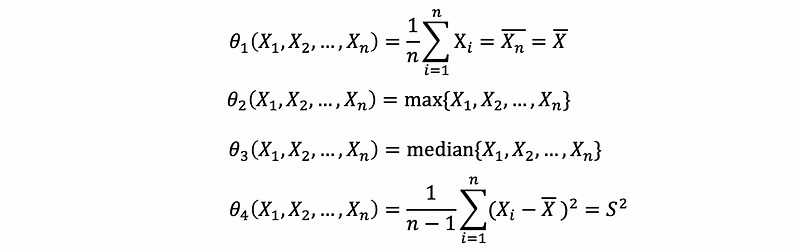
So how do I find good statistics, for example, statistics that are useful for estimating underlying population parameters?
(6) The Definition of Population Parameters
The population parameters governing a random variable are just those parameters that fully determine its distribution (aka. CDF).
- Normal Distribution

- Stable Random Variable

- Exponential Distribution

- Bernoulli Distribution

So the thing we should keep in mind here is the idea of the platonic form: there is a true world and it has perfect form and humans can quite access to it or see it, which, under a religious view, we may say “God knows” and maybe only god really knows what these parameters are and we don’t know, but we can take a peek of them through collecting data and estimating.
If we want to, for example, suppose that incomes follow an exponential distribution with parameter λ, the question may be what is the true λ. There is actually an ideal λ and it does exist, but it is never accessible. So we have to estimate it through a collection of data or using statistics, and usually, we asked about the uncertainty of the estimates so that we end up building confidence intervals, which will be a topic in the following sections.
(7) The Definition of Likelihood Function
Suppose that Xi is a random variable with density fXi(θ; xi). This notation of density function is an evaluation depending on two collections of variables. One is the actual position on the x-axis, order through X1, X2, X3, … in real space while you are evaluating the density function. But the other thing that influences the density function is the statistics or parameters that control it. So in case of a normal distribution, there are three things that define a normal density, we get to tell an x-location where you would like to evaluate, you have to tell μ and you have to tell σ². So θ is intended here in the density function to represent the parameters that control the density and xi’s is a particular location of x the x-axis.
For a random sample X1, X2, …, Xn with common density fXi(θ; xi), i = 1, 2, …, n, the likelihood function is defined as,

And because the random variables X1, X2, …, and Xn belongs to a random sample (X1, X2, …, Xn), then by definition we can know that all these random variables are independent. Thus, we can then have,

which is also,

the second expression is because all the Xi’s follow the same density function, so we don’t have to distinguish each density f with a subscript Xi, and we can just eliminate the subscript and use f for each of random variables.
(8) Maximizing the Value of Likelihood Function
Let’s say that Yale draws 10 random variables and she knows that the random variables are from an exponential distribution. The god secretly knows that the parameter λ of this exponential distribution is 1/3 and the mean of a sample from this distribution is quite around 3 (by the property of exponential distribution).

So if Yale would like to use a density function to describe these data in the bast way, it is okay to choose any λ as a parameter even though the result may be poor. What she can do on her best, is to choose a θ with which the density function best describes the density of the data. From the definition above, if we want to have a maximum probability density given parameter λ as a variable, what we can do is to maximize the likelihood function and then derive λ when the likelihood is maximized.

So the definition is that suppose we have a random sample X1, X2, …, Xn. You regard it as fixed. How do you choose a θ that best comports with, or is most compatible with these data? The answer is to choose a θ that maximizes,

so, we will choose,

The notation of ^ on any parameters or functions is the thing that we estimate or guess, not the real value based on the population.
(9) Log-likelihood Function: A Simpler Solution for Differential
Maximizing or minimizing a function that is the product of functions is yucky. (Why?) Because it requires the use of the product rule or maybe the chain rule as well, which can be sloppy.

We would like things to be more elegant and simpler compared with the differential rules, so what’s going to be the solution here? Or something that we don’t have to use the product rule, but something much much easier than that?
The solution is to use a log-algorithm! So the likelihood function with log outside (based on the log-algorithm) is so-called the log-likelihood function. It is defined by given the log-likelihood of random sample X1, …, Xn, given θ, is the function as,

Note we mean that the log process is legal if we get the same result of estimated θ when we do maximization to both L (argmax L)and l (argmax l), and, argmax L and argmax l are equivalent to each other. The reason why can this log process be legal for our likelihood function is that this guy log(x) is an increasing function (aka. non-decreasing function).

In short, we can say that this is legal because the monotonic increasing functions do not change the value of their extrema.
(10) The Definition of Maximum Likelihood Estimator (MLE)
For a random sample X1, X2, …, Xn (i.i.d. sequence of random variables, i.i.d is the abbreviation of “independent identical distribution”) with common density f(θ; Xi), we call,

the maximum likelihood estimator (MLE) for statistic θ.
(11) Steps Of Doing Maximum Likelihood Estimation
- Form the likelihood function L
- Create the log-likelihood function l
- Compute the partial derivatives with the respect to each unknown parameter
- Set each resulting expression equal to zero
- Solve the resulting equation or set of equators to identify critical points
- Use second-order conditions (i.e. a second derivative test, e.g. might need to use Hessian) to determine which critical point is maximum. (Possibly need to check endpoints)
(12) Maximum Likelihood Estimation on Normal Distribution
Suppose that X1, …, Xn is a random sample from a normal distribution with unknown mean μ and known variance σ², we can calculate the estimator of μ based on the steps above. We won’t go into any details here, but the conclusion of this is going to be,

Moreover, if you solve the same problem with σ² unknown as well, you will find the following joint solution as,

But it is not what we normally saw for an estimator of the variance. While actually, what the MLE for variance is not the exact formula that we are going to use for sample variance as,

This is because the MLE produces possible statistics that may not be the “best” in some way, for example, they could be biased. So because those statistics produced by MLE is not unbiased, the bias adjustments may be required here.
2. Central Limit Theorem
We now know how to find (possible good) statistics. We might like to know things about them. For example, their distributions. It turns out that the CLT (Central Limit Theorem) plays a key role in describing the distribution of statistics like the distribution of the random variable

(1) The Definition of Central Limit Theorem
Suppose that X1, …, Xn is a random sample, for example, an independent identically distributed sequence of random variables.
Call the common mean μ of the random variables μ = 𝔼[Xi].
Call the common finite variance by σ² = Var(Xi)<∞.
For large n (i.e. as n tends to infinity), the following results approximately hold,

or,

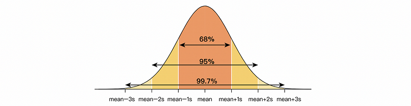
(2) Empirical Rule of Symmetric Interval
On a normal distribution, about 68% of data will be within one standard deviation of the mean, about 95% will be within two standard deviations of the mean, and about 99.7% will be within three standard deviations of the mean.
(3) Central Limit Theorem: An Example
Suppose that 88 people draw 88 Xi ~ Exp(2), and each of them independently draws exactly one Xi. So,
(a) What is the approximate distribution of ΣXi?
Ans: Based on the CLT, the sum of the random variables Xi ~ Exp(2), ΣXi, which is also a random variable, follows the normal distribution.
(b)What’s the mean, variance, and the standard deviation of ΣXi?
Ans: because we have,
So,
- Mean = n/λ = 88/2 = 44.
- Variance = 2n/λ²=88/4=22
- Standard Deviation = sqrt(Variance) = sqrt(22)
(c) Using the Empirical Rule, which symmetric interval would be expected to find ΣXi in 95% of the time?
Ans: Based on the Empirical Rule, approximately 95% of the time the random sum ΣXi will be in the interval [44–2sqrt(22), 44+2sqrt(22)].