Probability and Statistics 7 | Acceptance Rejection Method
Probability and Statistics 7 | Acceptance Rejection Method

- Acceptance Rejection Method
(1) Recall: Computable Inverse CDF
For the method of inverse transforms, one of the things that we should recall is that we needed a computable inverse of some cumulative distribution function.
(2) A question to Think About: What if there’s no easily inverse of the given CDF of the target random variable?
We can use the acceptance-rejection method in order to deal with these kinds of problems. So basically, the acceptance rejection method is a method that we used when the CDF or the inverse of CDF is not possible to access.
(3) Auxiliary random variable
An auxiliary random variable is been chosen ideally so that it is easy for us to simulate random numbers. For example, you can use the method of inverse transforms because there is a computable inverse.
(4) The Context for Acceptance Rejection Method
- Target a random variable X and its PDF f

- Auxiliary random variable Y and its PDF g

- Generate a random tuple (x, y) under the space of g. Then there can be two results, the first will be this dot is created between f and g, and another is that this dot is underneath both f and g. For example,
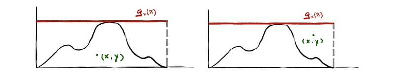
- Then, compute f(x) and compare it with y. If f(x) < y, we reject this dot. Else if f(x) > y, we accept this dot.

(5) The Definition of Realization
The realization of a random variable is an observed value, which is the value we actually observed form that random variable.
(5) The Acceptance Rejection Method Algorithm
- Simulate a realization u of random variable U ~ Unif(0, 1)

- Independently, simulate a realization y from Y, the auxiliary random variable with PDF g

then we can have,
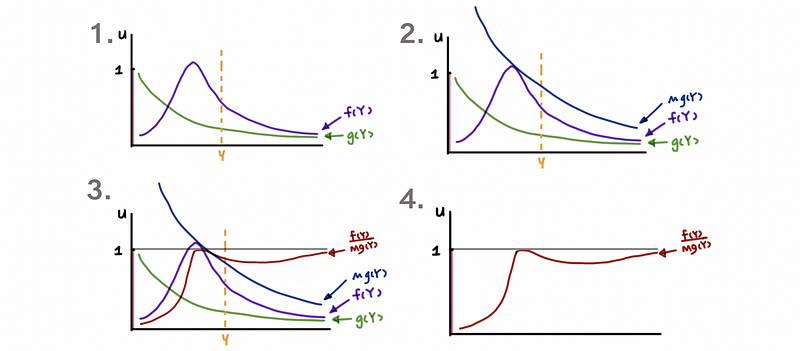
- If u < f(y)/Mg(y), then accept u as a realization of random variable X; if not then reject u and back to the first step
Note that the constant M is usually chosen as the largest value attained by f(x)/g(x) over the support set A of random variable X and random variable Y. It is the same meaning of M is the supremum (least upper bound) of f(x)/g(x).

The only condition for this algorithm to be true is that the probability of Y ≤ y given U ≤ f(Y)/Mg(Y) is the same as F(y). It is written as,

So we have to prove this.
(6) The Proof of the Acceptance Rejection Method
Suppose we define the event A and B as

by,

then we have,

the random variable Y has a density g, and suppose the CDF of random variable Y is G, by definition we can derive,

It is also that,

then,

then,

then,

then,

so we can have,

there is also,

so that,

then,

then,

then,

then,

thus,
