Probability and Statistics 8 | The Student’s T Distribution For Small Sample, Chi-Square…
Probability and Statistics 8 | The Student’s T Distribution For Small Sample, Chi-Square Distribution For Variance, and Confidence Interval

- The Student’s T Distribution
(1) The Standardized Center Limit Theorem
Note that if CLT says that for large n, we have that,

then, this also means that,

(2) The Weaken Condition of Standardized Center Limit Theorem
A weakening of the standard result is ( for example, when we don’t know σ ) is to replace σ by s, where s is given by,

This gives us a random variable, which is frequently noted as T.
(3) The Student’s T Distribution
Suppose we have an estimator of σ which is, as we have said, s, and by the standardized center limit theorem, we can then have, the random variable T satisfies,

we then call the distribution the student’s T distribution and the parameter (n-1) is called the degree of freedom in this distribution.

Note that the tails of a student’s t distribution are a bit flatter than a standardized Gaussian (Normal) Distribution. It is also a common result that as n → ∞, we have t( n-1 ) → N(0, 1)
2. Confidence Intervals
(1) Motivation For Confidence Intervals
All confidence-interval-like results come from some CLT-like results or some knowledge about the distribution of a statistic. Here is an example.
Let X1, …, Xn be a random sample from a normal random variable with unknown mean μ and known variance σ² (This is a quite strong statement and we are cheating here. So what we want is to give a brief example and we will talk about some general cases later). Under the CLT, we have the following result that if we choose a well-chosen threshold in the left tail of the standard normal distribution, and we find the probability is between that well-chosen threshold, then the probability will be exactly equal to 1-α,

Now, let’s take this expression and seek to isolate μ,

then,

then,

then,

(2) The Interpretations of Confidence Interval
Let,

and,

FALSE Interpretation #1:
(1-α)100% chance of the data lies between (i.e. Xi5) lie between a and b. This is simply false and the issue here is the confidence interval comes from a CLT result, which is a commentary on the distribution of statistics. By CLT, the quantile of the normal distribution is for the sum of these data, but not for the data themselves.
FALSE Interpretation #2:
(1-α)100% chance of the

(standardized) lies between a and b. This is also false. So what is the exact probability that the X-bars lie in the interval? The answer should be 100% because it constructed to do so. So this interpretation is equally bad with X-bar (standardized) lies between it 100% because a and b are determined by X-bar.
TRUE Interpretation #3:
There is a (1-α)100% chance that the true population mean μ lies between the random interval a and b.
- Objection
This interpretation suggests that μ is stochastic and, without th comment “random interval” downplays the notion that a and b are random endpoints.
- Assume Connection
The random interval a and b is constructed in such a way that contains μ 100(1-α)% of the time.
TRUE Interpretation #4:
The confidence interval over my particular random sample is [a, b]. Similarly constructed intervals, computed over many different random samples, contain the true population mean μ with probability 1-α.
(3) The Prior Confidence Interval
If,

is exact that if X1, …, Xn are normal and σ is known. But in practice, both of these assumptions are unrealistic, so we have to find a way to replace or remove these assumptions.
- Weakening Condition #1
If the Xi s’ are not normal — but are not severely non-normal — then the interval,
is approximate rather than exact (Justification CLT). So how approximate is depend on how much the Xi deviates from the normal distribution. If Xi ’s are severely skewed with a flat tail, then this is not going to be a good approximation. If Xi ’s are kind of like roughly symmetric with tails not too thin or too fat, then this is going to be a good approximation.
- Weakening Condition #2
If σ² is unknown and must be estimated with s², we end up with,

In general, we can make this approximation a little more exact by using,

instead of,

If we do that, and use,

this 100(1-α)% confidence interval is exact when the Xi are normal (but σ unknown) and an approximation otherwise.
(4) The De Moivre -La Place Theorem: Precursor for CLT when Xi ‘s are Bernoulli random variables.
Let Xi ~ Ber(p) be independent for i = 1, …, n. Call X = X1 + … + Xn (Aside: X ~ Bin(n, p) ), then,

in other words,

this means,

Aside, I will try to reserve π for the true population proportion and,

for the sample proportion.
(5) The De Moivre -La Place Theorem: An Example
By the standardized CLT, we can have that if we standard the statistic θ, then,

Suppose that we have π for the true population proportion and,
for the sample proportion. By DL Theorem,

then,

then,

so,

is the confidence interval for the 100(1-α)% probability of true value π.
(6) The Condition for De Moivre -La Place Theorem As An Approximation
So when is the approximation under DL good? There is a heuristic when

then we can say the approximate is just fine. This will be unhelpful if we don’t know π, so just use
to substitute π if we don’t know its exact value in the first place.
(7) Chi-Square Distribution
χ²(n) is, by definition, a random variable generated by summing squared independent standard normal random variables.
For example, if X⊥Y, and Z = X² + Y² and X ~ N(0, 1) with Y ~ N(0, 1), then Z ~χ²(2).
(8) The Confidence Interval for The Variance σ²
If X1, …, Xn are independently identical distributed (aka, i.i.d) normal random variables with mean μ and variance σ², then,

Using this result,

by graphing (χ² is a right-skewed distribution), which is,
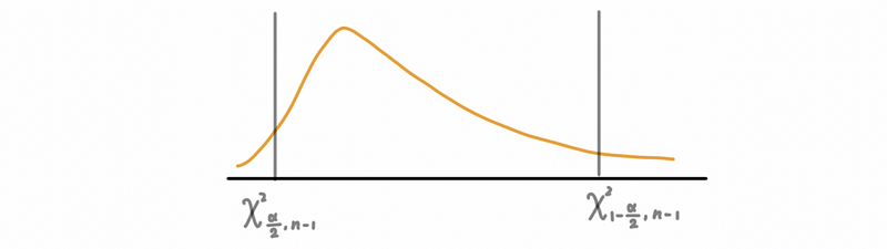
Then,

thus,

this is supposed to be our confidence interval for the variance.
(9) Conditions for Normality Assumption
For a theorem—like the one we just used or the student’s T theorem—how much abuse can normality assumption take?
As long as the random variable/data satisfy the following conditions, most results that we see in this class that depend upon the normality assumption are robust to its violation.
(a) No heavy tails for a random variable to no outliers for data drawn from a random variable
(b) No skewness, particularly severe skewness
(c) No multi-modality, i.e., you distributions should be unimodal
3. A Brief Review of Hypothesis Testing
Suppose that X1, …, Xn is drawn from a normal variable in an independent way. Suppose that you want to test H₀: σ² = 25 and H₁: σ² ≠ 25.
So our idea is that assume H₀ holds, which is also to say that if Xi ~ N(μ, σ² = 25), then,

We collect a random sample and take that n = 20 and we find that,

We can then calculate,

By calculating,

This tail probability .0074 = .74% encodes how rare it is to see a χ² ≥ 37.25 if H₀ is true.
We will talk more about that in the next part.