Relational Database 6 | Time Complexity, Index Algorithms Comparison for Searching
Relational Database 6 | Time Complexity, Index Algorithms Comparison for Searching

- A Quick Intro on the Big-Oh Notation and the Time Complexity
(1) Basic Assumption
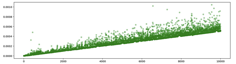
We can make an assumption (actually this is a fact but we are not going to prove this. If you are curious, you can study the assembly language) that the running time of a program has a linear relationship with the number of the executed lines (or problem size). We can easily see this relationship through the following program.
(2) The Definition of Operation Blocks
Because we have known that the running time of a program is positively related to the number of the executed lines N. Then we can write,

Suppose we define that an operation block is a block of several executed lines that will be looped, then we can have the relationship that the final number of the executed lines N is a function f of the number of executed lines in an operation block,

thus,

so that we can know the running time T is a function of the number of executed lines in an operation block, which can be defined as T(n).
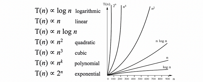
(3) Typical Time Complexity Curve
The expression of T(n) can be in various formations, typically, the time complexity curves can be,
(4) The Definition of Big-Oh Notation
Let f(n) and g(n) be nonnegative-valued functions defined on nonnegative integers n, then the function g(n) is O(f) (read: g(n) is Big-Oh of f(n)) if and only if there exists a positive real constant c and a positive integer n0 such that,

Actually, the big oh describes the upper bound of the time complexity.

Example #1. Prove that running time T(n) = n³ + 20n + 1 is O(n³).
Proof:

Thus, the running time T(n) = n³ + 20n + 1 is O(n³).
Example #2. Prove that running time T(n) = n³ + 20n + 1 is O(n⁴).
Proof:

Thus, the running time T(n) = n³ + 20n + 1 is O(n⁴).
Okay, now, then there seems like a conflict. Based on the examples above, we can know that the running time T(n) can be treated as both O(n³) and O(n⁴). So which one is the time complexity we would like to have?
For time complexity, we define that the lowest Big-Oh complexity or the lowest upper bound of the time complexity will be the notation that we use to describe the time complexity of an algorithm. Based on this definition, we can have the conclusion that O(n³) is our time complexity for the previous algorithm.
(5) The Dominant Term of Big-Oh Notation
The dominant term in a time complexity is the term that grows the fastest. Find the dominant term is the quickest way that we can calculate the time complexity of an algorithm. The common relationship of the terms is,
1 < log(n) < n < nlog(n) < n² < n³ < 2ⁿ
Example #3. Find the lowest Big-Oh complexity of the running time,

Answer:

then,

So n^(1.5) is the dominant term of the running time, and,

2. Time Complexity Example: Self-Balanced Binary Search Tree (AVL tree)
An AVL tree is a self-balancing binary search tree. We can see a visualization of this data structure from here.
(1) The Definition of the Height of an AVL Tree
A single-node tree has height 0, and a complete binary tree on k + 1 levels has height k. Suppose n is the number of the nodes that we have for an AVL tree, then the height h of this tree satisfies,

Proof:
See here.
(2) The Time Complexity For Searching the AVL Tree
At the worst case, we have to go to the deepest level of this tree in order to find the result we want. Then we have to do the search for h times and h is the height of this tree. Becasue h satisfies,

where n is the number of the nodes in this tree. Then the time complexity for searching an AVL tree is O(log n).
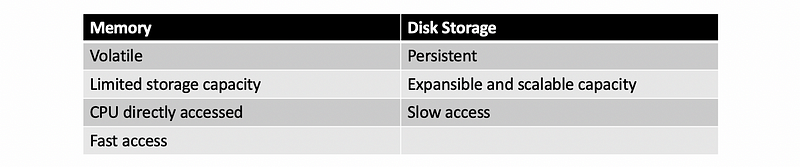
3. Memory vs. Disk Storage
4. Index Performance Comparison
In order to compare the performance between different algorithms, we have to define the table below,
B           # the # of pages
R           # the # of records per page
D           # the avg time to r/w to a disk page
C           # the avg time to r/w to a record
H           # the time to hash a record
F           # the fan-out (avg number of child for non-leaf nodes)
Then, (we don’t have to prove this)
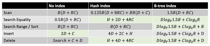
It is easy to find out that when a table is under construction (with new values keep updating to it), then it will be time saving if we remove all the indexes of this table. However, if the table is stable with no new values to insert, when we are going to conduct more sorted searching (ORDER BY) or range searching (WHERE a > b), then it will be better if we build a index of binary tree. When we are going to conduct more equality search (WHERE a = b), then we are going to build a index of hashing.
5. Index for SQL
- Create an index for the table
CREATE INDEX <indexname>
ON <tablename>
USING <indexmethod> (<colname>);
The index methods are,
btree (default)
hash
gist
gin
- Delete the index of a table
DROP INDEX IF EXISTS <indexname> CASCADE;
- Cluster the index of a table (btree)
CLUSTER <tablename>
USING <indexname>;
Note that a cluster btree will take more time to construct but it will perform better for searching and sorting.