Statistics for Application 2 | Confidence Interval, Moment Generating Functions, and Hoeffding’s…

Statistics for Application 2 | Confidence Interval, Moment Generating Functions, and Hoeffding’s Inequality

1. Confidence Interval

(1) The Definition of Statistical Significance (aka. α) for Normal Distribution

We define the statistical significance α for normal distribution as

We can use a plot to show this definition.

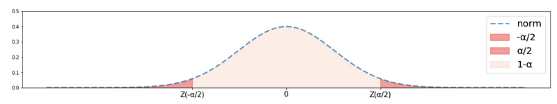
This is called statistical significance because when we are doing the hypothesis testing, what we are actually doing is to test whether or not some statistics are equal to 0 (which means these statistics are not important or two variables have no relationship). Because when the p-value is less than statistical significance, we can have enough evidence to reject the null hypothesis (statistics are equal to 0), so the result of these statistics must be significant.

(2) Pivotal Distribution

When we are trying to figure out the confidence interval, what we are actually doing is to switch the distribution under the data context to some distributions that we have already known. Then these distributions we known are called the pivotal distribution. We commonly denote the density function of a pivotal distribution as Φn(x) and we denote the density function of a standard normal distribution as Φ(x).

Based on the CLT, we have that,

Common pivotal distributions are as follows:

• Standard normal distribution
• Student’s t distribution
• Χ² distribution
• F distribution

If we don’t have a computer alongside with us, probably, we can randomly open a statistics textbook and find tables of this pivotal distribution in the reference.

(3) Pivotal Qualities (aka. pivots)

The pivotal quality is a function of observations and unobservable parameters such that the function’s probability distribution does not depend on the unknown parameters.

(4) Confidence Interval of Mean

Suppose we have only got one sample, and we have assumed that the number of random variables X1, X2, …, Xn in this sample is large enough for CLT. Then,

so we have,

then to solve μ, we have,

then,

This is the confidence interval of the mean value of any distribution of random variable X.

2. Moment Generating Functions

(1) The Definition of the Moment Generating Function (aka. mgf)

Suppose we have a random variable X and a constant t ∈ℝ, then, the moment generating function of X is denoted by Mx(t) as,

(2) The Moment Generating Function for Discrete r.v. X

Suppose we have a discrete random variable X, then its moment generating function is,

(3) The Moment Generating Function for Continuous r.v. X

Suppose we have a continuous random variable X, then its moment generating function is,

(4) The Meaning of the Moment Generating Function

The moment generating function is called so because we can use the moment generating function to find the moments of the distribution of a random variable X by taking the derivative of the MGF and evaluating the derivative at zero.

The first moment is,

thus,

Also, the second moment is,

then,

then,

then,

Thus, we can have that,

Then we could have a much easier and general way to calculate the statistics related to the moment (for example, the expectations, the variances, the standard deviation, and etc.).

(5) Moment Generating Function: An Example

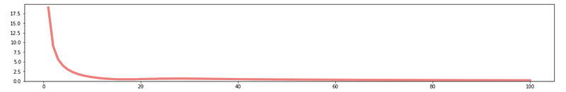
Suppose we have a random variable X ~ exp(λ), then the density function of this random variable X should be,

with X > 0.

then by definition of the moment generating function,

then,

then,

thus, this is equal to solve,

In order to solve this, because we have assigned the constant t ∈ℝ, now it’s time to make some constraints of it. Suppose we let t-λ < 0, which is also to say that t < λ. Then,

thus, we can have that, when t < λ ,

So,

also,

thus,

Therefore,

and,

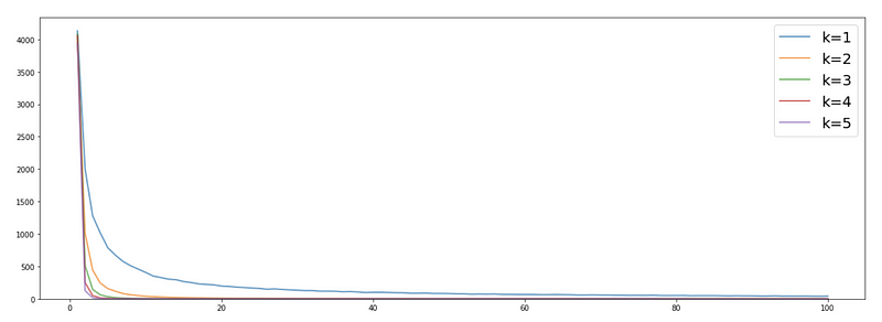
Note that the moment generating function of X is also,

then this is going to be a quick and easy way to calculate the k-th (k for any integer > 0) moment. We can find the mgf of the common distributions from Wikipedia.

3. Hoeffding’s Inequality

In the previous case, we have talked about the CLT when n is large enough, but what if we have a sample that is not that large and we can not say that it will tend to have the CLT. The answer is to use Hoeffding’s Inequality.

(1) Markov’s Inequality

Because when N is relatively small, the CLT no longer holds, so we have no idea about how the tails are going to look like. Actually, what we can do is to find the bound for the tails, and one of the most elementary tail bound is Markov’s inequality, which asserts that for a positive random variable X ≥ 0, with finite mean,

For example,

Proof:

Suppose we have a random variable X ≥ 0 and a positive number t,

then,

which is,

(2) Chebyshev’s Inequality

If we have positive random variable X ≥ 0 that satisfies,

then,

For example,

Proof:

By definition,

By Markov’s inequation,

therefore,

This is also,

(3) k-th Central Moment Chebyshev’s Inequality

This is very similar to Chebyshev’s inequality,

Proof:

(4) Recall: The Definition of Infimum and Supremum

Assume we have a constant p, for all ϵ > 0 and x ∈A satisfies,

then p is called the infimum of A and it is denoted as

Assume we have a constant p, for all ϵ > 0 and x ∈A satisfies,

then p is called the supremum of A and it is denoted as

(4) Recall: Infimum and Supremum vs. Minimum and Maximum

For a discrete finite set A,

(5) Chernoff Method

By Markov’s inequality,

then the 1st central moment Chebyshev’s inequality is,

Suppose we let,

then,

then, if we represent t as u and make t a new constant > 0,

then,

then, because the exponential function is an increasing function, then,

Because μ is a constant, so that,

then,

For many random variables, the moment generating function (we will talk about them later) will exist in a neighborhood around 0. This is to say that for some constant b > 0, the moment generating function is finite for all |t| < b. Because we also have that t > 0, thus the support set of t should be 0 < t < b. Then, if we choose to get a tighter upper bound, we can have,

this is also,

also,

This is called Chernoff’s method of the bound.

(6) Example #1 of Chernoff Method: Gaussian Tail Bounds

Suppose we have a random variable X ~ N( μ, σ² ), we have the mgf as

To apply Chernoff bound we then to compute,

By the fact that,

then,

then,

so that,

This is often referred to as a one-sided or upper tail bound of the Gaussian tail bound. We can check this by,

We can edit the times of trials N, μ, σ, and also u in this program to get the same output:

The inequation holds in {N} times trials

We can repeat the above calculation to obtain the analogous lower tail bound,

So to put these two pieces together, we can get the two-sided Gaussian tail bound,

(7) Chernoff Method Gaussian Tail Bounds and CLT

Suppose we have i.i.d. Gaussian random variables X1, X2, …, Xn ~ N(μ, σ²). We can construct the estimate:

When n is large enough, by CLT,

Thus, we can have the conclusion that,

However, when n is not large enough, this equation no longer holds. But by Chernoff’s bounds of Gaussian tail, we can have the bound of the tails. First of all, we know that,

then,

thus,

this bound works for all n’s.

(8) The Definition of the Hoeffding’s Inequality

By Chernoff’s bounds of Gaussian tail, we can have,

if we let,

then,

Suppose ΣX/n∈[a, b] (a < b and they are given numbers),

then, if we let u = t,

With some effort you can derive a slightly tighter bound (not going to prove here),

Thus, let n be a positive integer and X, X1, X2, …, Xn are independent and identically distributed random variables such that X∈[a, b] (a < b and they are given numbers). Let μ = 𝔼[X]. Then for all ϵ > 0, we have that,

This is called the Hoeffding’s inequality.