Time Series Analysis 1 | Introduction to Time Series, Moving Average Smoothing, Additive…
Time Series Analysis 1 | Introduction to Time Series, Moving Average Smoothing, Additive Decomposition, and Multiplicative Decomposition

- Introduction to Time Series
(1) The Definition of Time Series
A time series is a set of observations x_t of a time-dependent variable X_t at a specific time t. We can have discrete timepoints which are more commonly used, but we can also have continuously recorded time points that will not be covered in this series.
(2) Examples of Time Series
Next up, let’s see some of the time-series data examples,
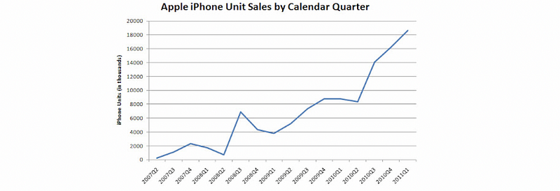
- Sales Data: iPhone Quarter Sales
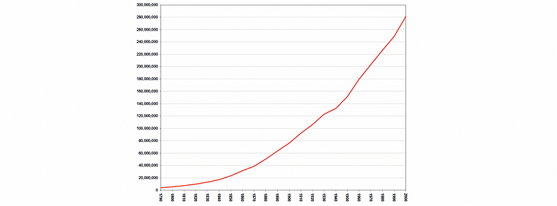
- Population Data: US Population from 1790 to 2000
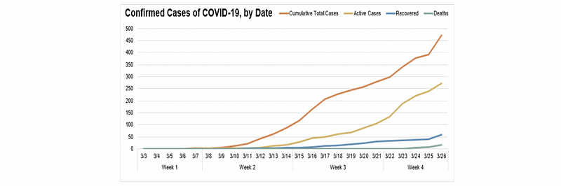
- COVID Data: infected number, death number, etc.
(3) Objectives of Time Series Analysis
Before we talk about the time series models, let’s first discuss the objectives of the time series analysis,
a. If we focus on the history of the data, we can do plots to examine the main features of the time series, and check particularly if there is,
- a general trend
- a seasonal component
- any noises
b. If we focus on the future, we can find a suitable probability model to represent the data so that it can provide,
- Interpretation of the given data: for example, what is the general trend for the unemployment rate, and what is just the seasonal component, and what might be accidental noise
- Forecasting: typically, there are two solutions for predicting the future using past data. These are statistical modeling that will be covered in this series and deep learning (i.e. DNN).
One example for the application of forecasting is weather temperature forecasting,

For the temperature forecasting, we can answer probably the following problems,
- Trend: is there a general trend of global warming
- Seasonality: is there a repeating cycle of seasonality
- Remaining Noise: are the noises correlated?
In conclusion, the statistical modeling approach is to model each of the components and then add them together. There are some
- ARIMA Model Family and Holt-Winters Exponential Smoothing: these are commonly used approaches because they give a higher weight to recent history. The benefit is that this approach is statistically and theoretically readable and understandable, but the downside is that these approaches are very hard to choose the proper parameters and estimate.
- Piecewise Linear Model: we can also choose some discrete points in the graph
- FB Prophet: a general case for forecasting everything developed by Facebook but it is not as flexible as the ARIMA family. The benefits are that (1) it has only a simple one-step setup; (2) it has the less computational burden
- Neural Network (DL or RNN): the RNN relies on lots of data, so it doesn't work well for univariate data but it works pretty well for the multivariate data on which the traditional statistical approaches don’t work well. For univariate data, there is actually a debate on if the RNN works better or if the traditional statistical approaches work better.
(4) The Definition of Time Series Model
In this series, we try to find a probability/mathematically model to fit the historic data and then use it to provide forecasting. A time series model for the observed data {x_t} is a specification of the joint distributions (or possibly only the means and covariances) of a sequence of random variables {X_t} or {X_1, X_2, …, X_t}, of which {X_t} is postulated to be a realization.
(5) Example of Time Series Models
Let’s now see some examples for the time series models,
- IID Noises: there is no trend or seasonality

- Broader Verison Noises: White Noises
A time series is a white noise if the variables are independent and identically distributed with a mean of zero. All variables have the same variance (σ²) and each value has a zero correlation with all other values in the series.

In order to prove a noise variable follows the distribution of white noise, we have to prove the following conditions.
a. 𝔼(X_t) = 0, ∀t
b. Var(X_t) = σ², ∀t
c. Cov(X_t, X_t+h) = 0, ∀t, ∀h≠0

- Regression Model: Trend model + White noise
a. Trend: m_t = a0 + a1t + a2t²
b. White noise: Y_t ~ WN(0, σ²)
c. Regression model: X_t = m_t + Y_t
- Fourier Components: Signal model (with seasonality) + Noise (don’t have to be white noise). An example is as follows,
a. Signal: s_t = cos(t/10)
b. IID Random Noise: Z_t ~ N(0, 0.25) (here we use a Gaussian noise)
c. Model: X_t = s_t + Z_t
(6) Common Types of Time Series Models
Finally, at the end of this part, let’s see some most commonly used models, which are also more complicated,
- ARIMA
- Prophet
- LSTM
All of them will be using the univariate use case, and we will discuss them in the coming articles of this series.
(7) Prediction Performance of Time Series Models
No matter what model you are using, you will hope that the future data go with the same pattern as your model. But in practice, things do not go that well. For example, the stock market data do not follow the time series model as we wish. So there are some metrics for the prediction performance, and we are going to cover them in the future sections.
2. Basic EDA
(1) The Definition of Time-Series Plot
The time-series plots are scatter diagrams or line diagrams of observations x_t against time variable t. These plots describe the general behavior of observations over time. A key difference that distinguishes the time-series plot and the regular scatter plot is that the date and time need to be datatime type.
(2) The Definition of Moving Average Smoothing Approach
When there are too many noises, sometimes the moving average smoothing approach can help to identify the trend. We should first choose a window size k, then estimate the moving average W_t at time t to be the average value of the k observations around time t.
In the book Introduction to Time Series and Forecasting, it uses the two-sided moving average, and here we focus on the pandas function
DataFrame.rolling(window = <WindowSize>).mean();
Basically, there is also another parameter center we can assign. The default value of it is False and we can assign it as True
DataFrame.rolling(window = <WindowSize>, center=True).mean();
Here is a possible result of moving average approach on the weather temperature when we have a window size of 30, 120, and 360.
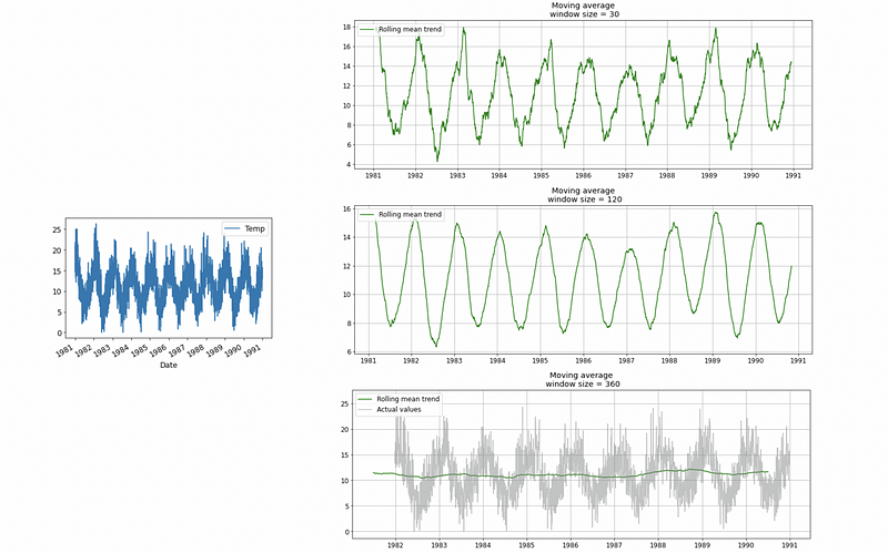
The basic calculation of the default moving average is that,

The calculation of the center moving average is that,

We can use MA smoothing to estimate trends, and it also provides a naive forecasting model.
(3) Choosing the Window Size Parameter k
When there’s mp seasonality we can try different k. When seasonality exists, if you want the trend to just present the general change without seasonality, then choose the size k equals the lag of seasonality.
(4) The Definition of Classical Decomposition
We have mentioned that there are three major components people try to identify when studying the time series data,
- Trend:
T_t - Seasonality:
S_t - Remaining noises:
R_t
The classical decomposition method originated in the 1920s. It is a relatively simple procedure and forms the starting point for most other methods of time series decomposition. There are two forms of classical decomposition, additive decomposition, and multiplicative decomposition.
(5) Additive Model Vs. Multiplicative Model
- Additive model: Additive model is useful when the magnitude of seasonal fluctuations or the variation around the trend does not change with time. As the name implies, the form of additive decomposition should be,

- Multiplicative Model: Multiplicative model is useful when the variation in seasonal pattern (or around the trend) appears to be proportional to time. This is a very common situation with economic data.

(6) Additive Decomposition Implementation
To perform an additive decomposition, there is something we have to decide,
- Generating de-trend data: Estimate the trend using MA smoothing (i.e. applying the MA filter on the data), and the window size k should be seasonal lag. For example, we can have the following window size as 365 for the weather temperature data. The series after MA smoothing should be the estimated trend series
T_t-cap. And the de-trended time series data should be,
X_t' = X_t - T_t-cap
- Estimating seasonality: Next, we should estimate seasonality under the assumption that the same seasonality repeats for the same cycle. The result of this averaging approach is the estimated seasonal series
S_t-cap. So for each season i, we have estimated valueS_i-capas

where N is the number of season cycles we have for the data
- Computing Noise: Finally, because we only have three components in our additive model, we can generate the estimated noise series
R_t-capin this model,
R_t-cap = X_t' -S_t-cap =X_t - T_t-cap -S_t-cap
(7) Multiplicative Decomposition Implementation
The implementation of multiplicative decomposition is quite similar to additive decomposition. Again, we should consider the following steps,
- Generating de-trend data: Estimate the trend using MA smoothing with window size k. But the de-trended time series data should be,
X_t' = X_t / T_t-cap
- Estimating seasonality: for each season i, we have estimated value
S_i-capas,

- Computing Noise: Finally, because we only have three components in our multiplicative model, we can generate the estimated noise series
R_t-capin this model,
R_t-cap = X_t' /S_t-cap =X_t / (T_t-cap *S_t-cap)
(7) Problems for Addictive/Multiplicative Decomposition
- Over-Smooth and Potentially Unrobust: The trend estimate
T_t-captends to over-smooth at the rapidly rising or falling points. So when we have some unusual values in a small number of periods, the models are not robust. - Seasonality Existence Assumption: The classical decomposition assumes that the seasonal component exists in the model even if there’s not
- Repeated Seasonality Assumption: The model assumes that the seasonal component repeats for each cycle, which can be violated
(8) Models to Fix These Problems
Based on the previous problems, we have generated several models to fix them.
- STL: modeling the seasonal and trend decomposition with LOESS regress curve
- etc.