Time Series Analysis 5 | Partial Autocorrelation Function and Plots

Time Series Analysis 5 | Partial Autocorrelation Function and Plots

1. Partial Autocorrelation Function (PACF)

(1) Recall: ACF Plot for AR(p) and MA(q)

• AR(p): for stationary AR(p), it can be written as an MA(∞). Because the ACF plot of MA shuts off at q so that an MA(∞) ACF plot should never shut off theoretically. So the ACF plot may decay slowly and hard to judge sometimes.

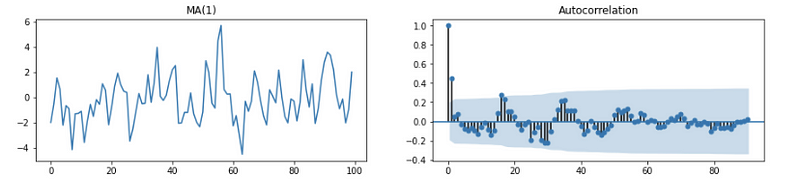
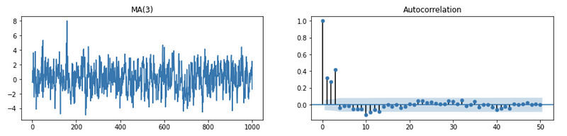
• MA(q): Theoretically, MA(q) is a q-correlated process and should have 0 ACF when h > q. ACF plot should shut off quickly and where it shuts off can give an estimate of q. For example, we can examine that the following ACF plot shut off at h = 2, so we can estimate this is a MA(2) process.

(2) Recall: The Definition of Autocorrelation Function (ACF)

ACF is the complete autocorrelation function where all X_t’s are random variables,

(3) The Definition of Partial Autocorrelation Function (PACF)

While PACF is the conditional autocorrelation between X_t and X_{t+h} when x_{t+1}, …, x_{t+h-1} are fixed.

(4) Simplified Version PACF

Although this formula looks very challenging to estimate at the first glance, Brockwell and Davis (1991) showed in their book that PACF is equivalent to the correlation between the following two prediction errors,

And,

where P is the prediction operator that is used to estimate X_t and X_{t+h} by using the condition of fixed X_{t+1}, …, X_{t+h-1}. For example,

This is to say that the PACF for {X_t} is also,

(5) Calculating PACF 1: Using Regression Residuals

Based on the simplified version of PACF, we can generate two approaches to estimate PACF. The first approach is to calculate PACF based on the two regression residuals.

• Fit the first OLS regression, then get the residuals Ɛ_{t+h}

• Fit the second OLS regression, then get the residuals Ɛ_{t}

• Then calculate the sample correlation between two sets of residual as the sample PACF. So the PACF(h) should be equivalent to,

However, this estimation does not look the same way as the practical models, so they figure out some ways to improve it.

(6) Calculating PACF 2: Yule-Walk Method

Yule-Walk method is the default method used in Python, and we have to discuss it here because it gives a more accurate estimate of PACF. The basic idea is that the correlation coefficient of X_{t} and X_{t+h} should be equal to the parameter of the OLS regression estimation between them.

Therefore, this method understands the conditional Corr(Xt+h, Xt) as,

where β_h measures the proportion of the variance in X_{t+h} that is explained by X_{t}, and we can use it as an estimate of the value of the partial correlation.

Note that the expression above can also be written

This can be written in the form of an AR(h) model,

And,

To get this coefficient, we have to multiply this equation,

On both of its sides by X_{t-1}, X_{t-2}, …, X_{t-h} respectively, and then take the expectation,

In matrix form, we have,

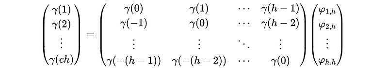
This can be written as,

Which is also,

Therefore, the estimate PACF(h) should be,

(7) Levinson-Durbin Recursion Algorithm

Now, let’s discuss how can we calculate the inverse matrix of the least square coefficient covariance matrix. As our discussion, we can find out that the covariance matrix Γ_h is a Toeplitz matrix, which is defined as each of its descending diagonal from left to right is constant.

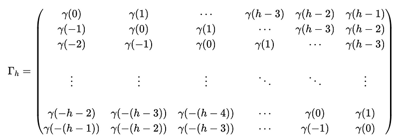
For the Toeplitz matrix, we can apply the Levinson-Durbin recursion (which has a complexity of Θ(x²)) for calculating its reverse instead of the Gaussian elimination (which has a complexity of Θ(x³)). You can find out how we do Gaussian elimination by,

In scipy.linalg package of Python, the ordinary solve method calculate the inverse matrix by Gaussian elimination and the solve_toeplitz method calculate the inverse matrix by Levinson-Durbin recursion. For example,

import numpy as np
from scipy.linalg import toeplitz, solve, solve_toeplitz

c = np.array([1, 3, 6, 10])
r = np.array([1, -1, -2, -3])
T = toeplitz(c, r)
I = np.identity(4)

# Solve by Gaussian Elimination
inv_gaussian = solve(T, I)
# Solve by Levinson-Durbin recursion
inv_levinson = solve_toeplitz((c, r), I)

# Check the result
print("Gaussian:\n", np.abs(np.round(np.dot(T, inv_gaussian))))
print("\nLevinson:\n", np.abs(np.round(np.dot(T, inv_levinson))))

And the output should be,

Gaussian:
 [[1. 0. 0. 0.]
 [0. 1. 0. 0.]
 [0. 0. 1. 0.]
 [0. 0. 0. 1.]]

Levinson:
 [[1. 0. 0. 0.]
 [0. 1. 0. 0.]
 [0. 0. 1. 0.]
 [0. 0. 0. 1.]]

2. PACF Plots

(1) Recall: ACF plots for MA

Recall the ACF plots for MA(1) as we have discussed in this article,

Also, for MA(2), we can have,

Continue this process for MA(q), we can find out that

So the ACF plot of a MA(q) process should shut off at h = q. For example,

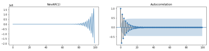
However, the ACF plot for AR doesn’t imply any information about the order (only decaying) and we ought to find another way out.

(2) PACF plots for AR

PACF plot, instead, helps with identifying the AR(p) process and gives a suggestion for p. Let’s first see how it works.

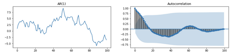
For AR(1) process, we have,

When h = 0, the PACF of this process should be,

When h = 1, the PACF of this process should be,

When h = 2, we have,

And for the first expression, we have,

And for the second expression, we have,

Therefore, we have,

This is,

Because noises {Z_t} are uncorrelated, we can then have,

Therefore, we have for MA(1),

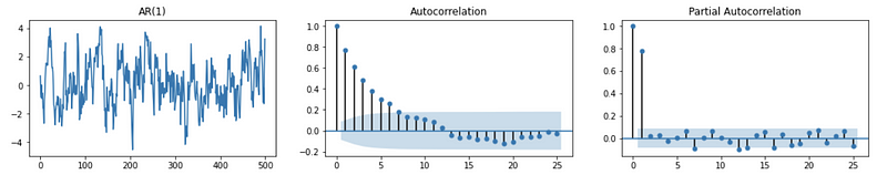
In general, for a AR(p) process, the PACF should be,

So the PACF plot of an AR(q) process should shut off at h = q. For example,

However, the PACF plot for the MA process is only decaying, and hard to tell where it shuts off. Note that if both the ACF plot and the PACF plot are decaying or shutting off, probably we are doing a combination of the ARMA model.