Time Series Analysis 6 | ARMA Estimation and Forecasting

Time Series Analysis 6 | ARMA Estimation and Forecasting

1. Stationary AR(p) and Invertible MA(q)

(1) Recall: The Definition of AR(p)

Or,

(2) Recall: Stationary Condition of AR(p)

AR(p) is able to use for stationary data should be,

• For population: The roots of Φ(x) = 0 should lie outside the unit cycle of |x| ≤ 1 (i.e. this means we should have all roots |x| > 1).
• For a sample: ADF test

(3) Recall: The Definition of MA(q)

Or,

We don’t have any condition for the MA process to be stationary.

(4) Problem of Estimating MA(q)

Although we don’t have to show a MA process is stationary or not, the MA process has some problems with its estimation.

• Suppose we are given {X_t}, then we don’t have any actual observation on the noise {Z_t}.
• When we use MLE to estimate an MA(q) process, there are cases that we have up to 2^q local optimations.

This is to say that if we have a certain MA process, we can not estimate it if we don’t constrain it with some conditions.

(5) Invertible Condition of MA(q)

To make an MA process estimatiable, we have to add a condition. And as we have discussed that an AR(p) process can be written as an MA(∞) process, the MA(q) should also be able to be written as an AR(∞) process. Based on this idea, if we can rewrite an MA process to an AR process, we must then be able to make some useful estimations.

Recall that an MA(q) process should be,

Then if we can estimate by it (i.e. it has an invertible generating function), it can be written as,

If we write the inverse of generating function as a convergent series expression, we can then have an AR(∞) process.

So the invertible condition for MA(q) is that if the zero roots of the generating function Θ(B) are all outside the unit circle |x| ≤ 1 (i.e. this means we should have all roots |x| > 1), we should be able to confirm that this MA(q) is invertible.

2. ARMA Process

(1) The Definition of ARMA Process

Now that we have discussed the AR process and the MA process, let’s continue to discuss the ARMA process. {X_t} is an Autoregressive Moving Average Process (ARMA) with order p and q if,

This can also be written as,

With the generating functions, we can have,

where,

All ARMA models we are going to use for fitting data are assumed to satisfy the stationary condition (causality) for generation function Φ(B) and invertible condition for generation function Θ(B).

• Stationary (like MA)

• Invertible (like AR)

(3) ARMA Fitting Process

In practice, if we identities the stationary condition of data from the plots and tests, what are the steps to take in order to fit the model ARMA(p, q)?

• Order selection: If we have only an AR process or MA process, then we can get a suggested order from the ACF plot or the PACF plot. However, if we need to fit a general ARMA(p, q) process, we should start from different pairs of p and q, and then choose the one with the smallest AIC or BIC on the whole dataset. Then we should use metrics for prediction performance as RMSE, MAE, or MAPE with cross-validation and train-test validation. We are going to talk about this later.
• Model Estimation: Generally, we are going to use MLE + recursive algorithm (for searching) for this problem. The recursive algorithm is Kalman-filter Recursive Algorithm (aka. MLE-CSS) in Python. In an ARMA model, we have to estimate the following (p + q + 1) parameters,

• Forecasting

(4) Estimating ARMA(p, q)

So now what we have to do is to estimate all the coefficients of an ARMA(p, q) model and the likelihood function should be,

Although the distribution assumption doesn’t matter for a log-likelihood result, the commonest one is a Gaussian distribution. So we will have,

where the covariance matrix should be,

Note that the mean of this distribution doesn’t necessarily need to be 0, because we can shift the data up or down.

So the likelihood function with MVN assumption should be,

And our goal should be,

And we can denote this as,

(5) MLE-CSS Method

In order to maximize the likelihood function of this ARMA process, we have to find a way on calculating the determinate of Γ_{n+1} and the inverse matrix of Γ_{n+1}. Let’s first have these two definitions,

• The Prediction Error

• The Mean Square Error

Also, we have to make an assumption of,

Because there is no previous data to be used for estimate X_0 X_0-hat. So for the estimate of X_1 X_1-hat, we can have,

Then,

For the estimate of X_2, we can have,

Then,

Continue and we can finally have,

In the matrix form, we can have,

where,

We can find out that the A_n matrix is a lower triangular matrix and this matrix is invertible if and only if no element on its principal diagonal is 0. Based on the format of A_n, we can say that A_n is an invertible matrix. So,

Because by definition of prediction error,

We can then have,

which can be written as,

And the Λ matrix should be,

So we have,

• The estimate of X_{t} can be calculated by using the residuals from the previous steps (i.e. the observed values and the estimated values).
• In each step, we can update the model and the coefficients λ’s.

But how to calculate λ’s? In fact, the coefficient λ’s can be calculated recursively with MSE ν_{t+1} by,

• Starting from,

• Then,

• And,

This algorithm helps reduce the MLE by,

And the sum of squares should be,

where,

So the likelihood function is then equivalent to,

Now, let’s check back our basic assumption,

And we can find out that this can be violated in many practical cases. If the mean is not zero, we have the ARMA model on the centered data and the noise doesn’t change. So in Python, we assume the expectation of {X_t} equals to the sample mean,

So we have the ARMA model as,

(6) ARMA Forecasting

To forecast an ARMA model, we have to use the previous residuals to estimate noises. For example, for an ARMA(2,1) process,

For X_1, we can not go back the whole way because we only have 1 historical data point X_0.

Continue, we have,

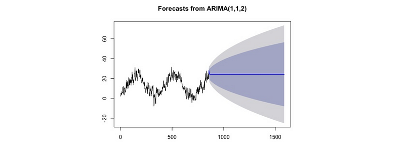
This is the end of our sample, but we can also continue this for forecasting by the out-of-sample data (i.e. estimated data). However, we will finally lose the support of the real historical data, and the changes will become smaller and smaller. So an ARMA model is good at predicting the short-term future but bad at predicting the long-term future, and long-term forecasting tends to become flat. The more reliance on the previous data, the quicker the forecasting becomes flat, this is because if the time series does not exhibit any obvious structure, like trend or seasonality, a flat line of mean is the best forecast. You can find an example here.