Time Series Analysis 7 | ARMA Model Selection

Time Series Analysis 7 | ARMA Model Selection

1. Order Selection

(1) Recall: AIC and BIC

We have discussed AIC and BIC in the linear regression series, and now let’s review them before we continue. AIC and BIC metrics choose the model with the largest log-likelihood with a penalty term on the number of estimate parameters.

• Akaike Information Criterion (AIC)

• Bayesian Information Criterion (BIC)

where, for an ARMA(p, q) model, k should equal to,

Also, n in BIC is the number of observations.

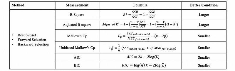
Because they are both model selection metrics, we can also refer to the following table,

(2) Properties of AIC/BIC for Model Selection

• BIC tends to choose simpler models: This is because n ≫ e² ≈ 8.
• Generality: They can protect us from overfitting by constraining the number of parameters.
• No need for train-test splitting: the whole data gives the best estimate of the likelihood.
• Only works for the same model family: for example, we can compare an ARMA(1,2) process and an ARMA(2,3) process, but we can not compare an ARMA(1,2) process to a Prophet model.

(3) Train/Validation/Test Sets

For a given dataset, we have to split it for performance measurements.

• Train Set: used for fitting the model
• Validation Set: used for evaluating forecasting performance of different models and then select the model with the smallest prediction error
• Test Set: Measure the performance of the final model by pretending the testing observed values are unknown

(4) Prediction Metrics for Cross-Validation

We have discussed that AIC and BIC work the best for the whole dataset, but commonly we would like to measure the performance of the cross-validation. Therefore, there have to be some other prediction metrics.

• Root Mean Square Error (RMSE)

For a training set of X_0 to X_m and a validation set from X_{m+1} to X_{n} , we have,

• Mean Absolute Error (MAE)

For a training set of X_0 to X_m and a validation set from X_{m+1} to X_{n} , we have,

• Mean Absolute Percentage Error (MAPE)

We should keep in mind that using different metrics might result in a different model.

Another problem is that why don’t we choose R² as a metric for time series cross-validation? This is because R² is calculated only by the training set (i.e. SSE shows how well the training results fit the real data) and it gives no information of the validation set. So a higher R² doesn't show anything about whether the model makes good forecasts.

(5) Rolling Forward Cross-Validation

In practice, it is rare to see just one train-validation set and commonly we don’t choose the training set and validation set randomly. Basically, we can conduct a rolling forward cross-validation.

• Rolling one-step forward Cross-Validation

Let’s suppose we have a dataset {X_t} of seven observations.

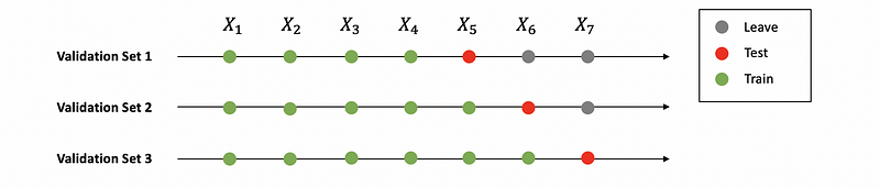
Based on this figure above, we can generate three train-validation pairs,

Train = [X1, X2, X3, X4]; VALID = [X5]
Train = [X1, X2, X3, X4, X5]; VALID = [X6]
Train = [X1, X2, X3, X4, X5, X6]; VALID = [X7]

Here, the rolling window is 1.

• Rolling two-step forward Cross-Validation

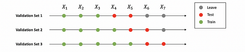
Based on this figure above, we can generate three train-validation pairs as

Train = [X1, X2, X3]; VALID = [X4, X5]
Train = [X1, X2, X3, X4]; VALID = [X5, X6]
Train = [X1, X2, X3, X4, X5]; VALID = [X6, X7]

We should change the rolling window k based on how it performs in short term and long term.

(6) Cross-Validation Coding Template

For rolling forward cross-validation with window 2,

Train, Test = Test_Train_Split(X)
Train_i = Train

Loop from i = 0 to (n-m):
    Model = ARIMA(Train_i)
    Train_i = Train + i   
    y-hat_1 = Model.forecast(2)[0]
    y-hat_2 = Model.forecast(2)[1]

Test_1 = ...
Test_2 = ...

RMSE_1 = foo(Test_1, y-hat_1)
RMSE_2 = foo(Test_2, y-hat_2)