Time Series Analysis 8 | ARIMA and SARIMA Models

Time Series Analysis 8 | ARIMA and SARIMA Models

1. ARIMA Model

(1) The Definition of ARIMA Model

The Autoregressive Integrated Moving Average ARIMA(p, d, q) Process models a non-stationary time series {Y_t} that can be decomposed into an approximate polynomial trend m_t and stationary remaining R_t. So,

where m_t is a polynomial with d terms,

If we differencing Y_t by d times, then we can get a stationary X_t defined as,

where B is the backward matrix for Y_t in this section, not for X_t.

Proof: when d = 1,

Then,

Then,

So,

So {X_t} is stationary.

When d = 2,

In this case, {X_t} is also stationary.

(2) Expression of ARIMA Model

In summary, if we have an ARIMA time series {Y_t},

where,

Because by the definition of the ARMA model,

Then we have,

(3) ARIMA Example

Suppose we have an ARIMA model of,

Then we have Y_t as,

This is,

Although this process seems like an AR(2) process, it is actually not because this process is not stationary.

(4) Parameter Selection

• Find p and q: As we have discussed, if we want to find p and q, we should do auto-searchings based on AIC and BIC.
• Find d: We can decide the degree of differencing d based on the ACF plot and the PACF plot. Or we can keep differencing the time series data until ADF test shows stationary.

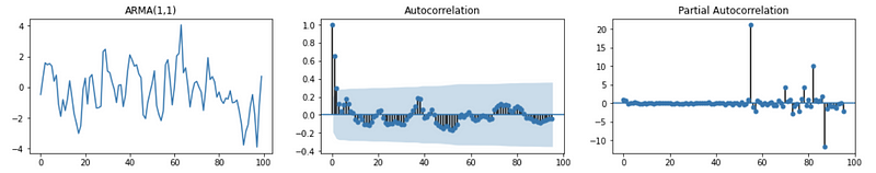
The ACF and PACF plot for an ARMA(1,1) model should be,

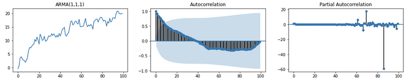
The ACF and PACF plot for an ARIMA(1,1,1) model should be,

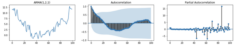
The ACF and PACF plot for an ARIMA(1,2,1) model should be,

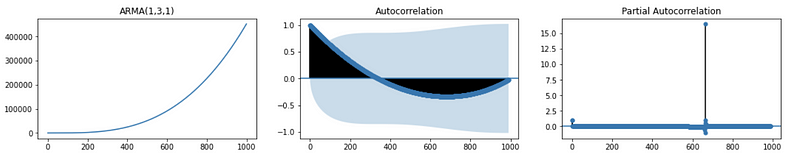
The ACF and PACF plot for an ARIMA(1,3,1) model should be,

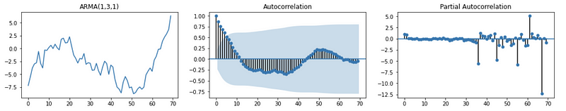
By this result, we can find out that the degree of differencing equals the number of the local maximum and the local minimum based on the ACF plot.

For example, we can first generate a simulated dataset simulated_data of ARIMA(1,3,1) data by,

import matplotlib.pyplot as plt
import numpy as np
from math import *
from statsmodels.tsa.arima_process import ArmaProcess
from statsmodels.graphics.tsaplots import plot_acf, plot_pacf

def plot_TS(title, TS, alpha=0.99):
    fig, ax = plt.subplots(1,3,figsize=(18,3))
    axes = ax.flatten()
    axes[0].plot(TS)
    axes[0].set_title(title)
    plot_acf(TS, ax=axes[1], lags=len(TS)*alpha)
    plot_pacf(TS, ax=axes[2], lags=len(TS)*alpha)
    plt.show()

ar = np.array([1, -0.5])
ma = np.array([1,0.2])
ARMA_object = ArmaProcess(ar, ma)
simulated_data = ARMA_object.generate_sample(nsample=1000)
trend = np.array([(15*x**3 - 1440*x**2 + 34200*x - 216000)/30000 for x in range(1000)])
simulated_data += trend
    
plot_TS("ARMA(1,3,1)", simulated_data, 0.99)

The plot printed should be,

Then the differencing function can be manually defined as,

def difference(dataset, interval=1, diff_deg=1):
    
    for j in range(diff_deg):
        diff = list()
        
        for i in range(interval, len(dataset)):
            value = dataset[i] - dataset[i - interval]
            diff.append(value)
            
        dataset = diff
        
    return diff

Then we can apply the difference function on the simulated_data with the differencing degree 1, 2, 3, and 4.

data_d_1 = difference(simulated_data, interval=1, diff_deg=1)
data_d_2 = difference(simulated_data, interval=1, diff_deg=2)
data_d_3 = difference(simulated_data, interval=1, diff_deg=3)
data_d_4 = difference(simulated_data, interval=1, diff_deg=4)

Then we should also define the function of the Augmented Dickey-Fuller test using the statsmodels.tsa.stattools.adfuller package.

from statsmodels.tsa.stattools import adfuller
import pandas as pd

def adf_test(timeseries):
    
    print ('Results of Augmented Dickey-Fuller Test:')
    dftest = adfuller(timeseries, autolag='AIC')
    dfoutput = pd.Series(dftest[0:4], index=['Test Statistic','p-value','#Lags Used','Number of Observations Used'])
    for key,value in dftest[4].items():
       dfoutput['Critical Value (%s)'%key] = value
    print (dfoutput)

The p-value on the differencing data with differencing degrees 1, 2, 3, and 4 of in my case should be (and you will generate a similar result),

deg-1: p-value                          0.994280
deg-2: p-value                          0.933897
deg-3: p-value                          1.236827e-29
deg-4: p-value                          0.000000

We can find out that, from this result, we will get a P-value ~ 0 when d = 3, therefore, we are able to conclude that the parameter degree. Note that different approaches may result in different conclusions and we have to use cross-validation + RMSE (or other metrics) to choose the parameters with the better prediction performance.

(5) Model Estimation and Forecasting

After choosing the parameters, we can apply the CSS-MLE method to estimate the ARMA(p, q) model based on the differentiated data to get an estimate X_t-hat. After that, the trend is forecasted based on the d we selected. For example, for d = 1, we have,

This is also,

2. SARIMA Model

(1) Trend Component (p, d, q)

The trend component is exactly the same as the ARIMA model, where we have,

• p: Trend autoregression order.
• d: Trend difference order.
• q: Trend moving average order.

(2) Seasonal Component (P, D, Q)_m

However, there are four more parameters we have to select because they are part of the SARIMA model,

• P: Seasonal autoregressive order.
• D: Seasonal difference order.
• Q: Seasonal moving average order.
• m: Seasonal lag, which is the number of time steps for a single seasonal period.

(3) General Form of SARIMA Model

Suppose we have a SARIMA(p, d, q)(P, D, Q)_m model and,

• D is the seasonality differencing degree for reaching stationary
• P is how Y_t is related to Y_{t-m} , Y_{t-2m} , … , Y_{t-Pm}
• Q is how Z_t is related to Z_{t-m} , Z_{t-2m} , … , Z_{t-Qm}

So we have,

where B is the backward operator for Y_t and X_t is a stationary time series.

And X_t can be modelized by,

Where,

And,

So the overall general form of a SARIMA(p, d, q)(P, D, Q)_m model should be,

(4) Parameter Selection

For additive model (i.e. seasonality pattern is independent to time), when D = 1 we have,

For the multiplicative model (i.e. seasonality pattern is sensitive to time), we should take a log-transformation on Y_t first to turn it in an additive model log-Y_t ,

Then we can apply D = 1 for log-Y_t as,

Here, we will only discuss the case when D = 1 and we can always choose D = 1 for any additive model or multiplicative model. Note that we don’t have to do trend differencing when D = 1 because the result (1-B^m) will include the case of (1-B).

The parameter m should be the same as the seasonality lag and we can choose it based on the time series plot and ACF plot.