Video Game Design 7 | Introduction to Game AI
Video Game Design 7 | Introduction to Game AI

- AI Movement and Steering Behaviors
(1) Chase/Evade Pattern
A common behavior pattern for the game AI is the chase/evade pattern. Suppose there are two characters in the game, the NPC and the User Controlled one.
- NPC: predator
- User Control: prey
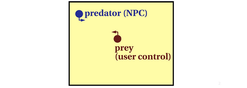
So now, we have to figure out the algorithm of the predator.
(2) Direction and Distance
To detect the position of prey, it is basically just leveraging the aspects of linear algebra.
- Relative Position Vector: The predator’s position vector subtract the prey’s position vector

- Direction: Normalize the relative position vector

- Distance: Modulus of the relative position vector

(3) Types of Movements
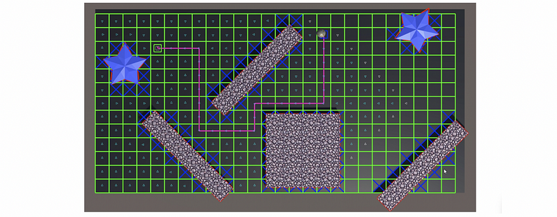
- Simple Movement: Orient agent velocity in the target direction. This can be very aggressive and the behavior doesn’t look natural. This movement is usually used for grid movement.

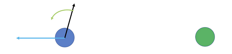
- Steering Movement: This movement to animate turns towards the target. It will also adjust the speed (e.g. slower when close to the target) to make the behavior more realistic.
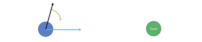
The steering movement can enhance the performance envelope, which means the behavior has constant acceleration and enforced max velocity for transactions and rotations.
- Fleeing Movement: Simply calculate the opposite ordered position vector.
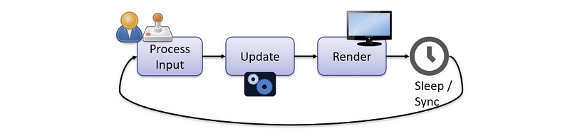
(4) Continuous Simulation
Also, we have to be mindful of continuous simulation in the nature of frame-based animation. With respect to the Unity platform, we have to be mindful of the time component when updating the velocity and so on because they are updated in the update cycles.
This brings us to the time dependency problem. We have talked about this problem before, and now let’s review it.
(5) Time Dependency
Time dependency is a problem that occurs because the frame rates in Unity demonstration are not constant. The Update function in the script is called once per frame, but the FixedUpdate function runs zero, once, or several times per frame based on how many physics frames per second are set in the time settings, and how fast or slow the frame rate is.
So to talk about its impact on the steering behavior, we used to think about using,

Instead, we should use,

(6) Prediction
We can keep on adding more features on the steering based on more use cases. And one feature we can add to the agent is the prediction of the target. Actually, there’s no need to calculate the precise intercept of the target because the target keeps moving and we will recalculate the prediction every frame. The calculation should be as follows,
- Distance:
Dist = (target.pos — agent.pos).Length() - lookAheadT:
lookAheadT = Dist/agent.maxSpeed - futureTarget:
futureTarget = target.pos + lookAheadT * target.velocity

There are also some traps for the prediction method,
- Extreme Predictions: very large lookahead t values
- Outta Map or Inside Obstacle Predictions: Could be spending your agent off the map or result in odd behavior. One solution for this is to clamp maximum map prediction, and the other one for this is to clip extrapolated future positions to fit on the map.
(7) Zero or Small Vector Problem
When the relative position vector AB is small or zero, we can get some undesired behaviors. Consider the situation of a vector normalization operation, the vector can become messier because the modulus of the vector is relatively small or zero. So we should be mindful about where the divided by zero problems crop up.
There are some solutions to this problem:
- Hold the current head and speed or perhaps a buffered sliding average of the last several measures
- Add a condition to decide upon an alternative steering strategy, for example, a state machine state transition that we will talk about later.
(8) Static Targets Problems
- Stopping Radius: Another scenario that we have here is arriving at static targets. If you are heading towards a target and you want to stop right on the target, you may not be able to do that based on a realistic performance envelope. So you actually need to detect when you are within a stopping radius (r). You are able to have the full speed outside the stopping radius. And the stopping radius is actually used for decreasing the velocity by distance from max to 0, abiding by maximum deceleration possible.
- Orbit Problem: If you are not planning on having your agent stop at the target, then what you need to do is to determine what the orbit radius is. Then the agent has to make a change to its current maximum term rate and its maximum forward velocity. They will just indefinitely orbit so the radius is easy to calculate.
(9) Obstacle Avoidance
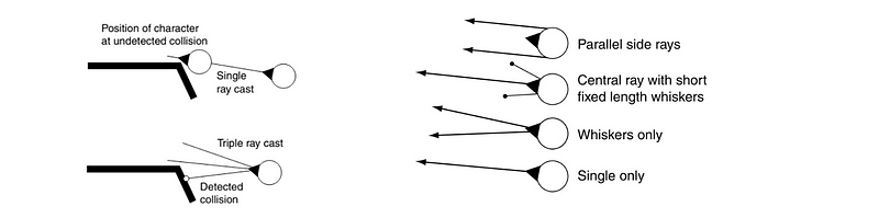
Next up, we will introduce a little bit of some other concepts to make our steering behavior agent more effective. So what we can do is to perform obstacle avoidance. This requires some sort of look-ahead window and generally, the simplest case is a raycast in the forward direction of the agent.

There are different probabilities for improvements of adding additional raycasts. The following diagram shows some patterns of the ray casts.
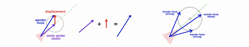
(10) Wandering
Another behavior that we would like to mention here is wandering. This is useful for non-player characters that are not violent. So maybe like someone in a town or in a role-playing game, you just want them to wander around aimlessly but not look unnatural. So rather than adding a random vector periodically to the agent, this approach works by placing an invisible wander radius ring in front of the agent (sort of like a carrot).
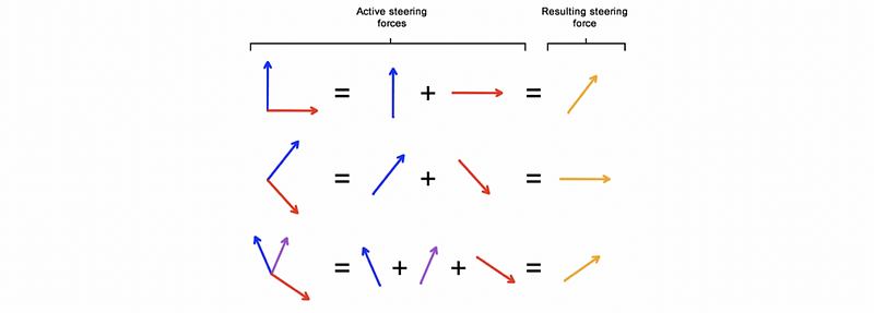
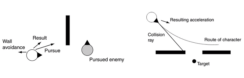
(11) Combination of Steering Behaviors
Sometimes we may have multiple steering goals, and the best approach to it is to use a combination of steering behaviors. Generally speaking, there are two kinds of combination,
- Simple Sum: we have to enforce the maximum speed
- Weighted Sum: weights can be based on some metrics like distance
However, there are some examples when things fall apart when you implement the combined steering behaviors, especially for the situation that the enemy runs behind an obstacle. The pursuing velocity combined with the wall avoidance velocity may generate some unwanted behaviors like detours. One solution to this situation may be that we don’t have to combine these steers at the same time. The agent has to make some higher-level decisions, and rather than continue to track the enemy from right to left and turning, it would be head just to the right of the obstacle until passing the obstacle. Then, they will have no worry about the turning.
In the extreme situation, if the steering behaviors are totally opposite, you may result in a zero or small vector, which we have discussed above. One result is that the agent can go back and forth forever, or it will be orbiting forever. We need higher-level control logic to deal with this problem.
(12) Motion Table for Blended Root Motion
So how can the agent select animation blend parameters that best direct its movement towards the steering target? Ultimately, what we need to do is to select animation parameters that will cause these different animation blends, and then the result is the root motion moment to release the frame. We could fit a function, but this solution becomes difficult for higher-order functions. Or we could create a lookup table. Finally, we can use this table to find animation parameters with the closest root motion to the steering target.
(13) Ballistic Projectile Aiming
Then, let’s discuss the topic of ballistic projectile aiming. This is a sort of behavior related to steering behaviors but it’s not exactly the same sort of issue. It is probably closest to prediction as we have discussed so far, but this is where we have non-instantaneous projectiles. So, it is not just like a raycast that hits you and makes you know that you have a hit. This is more like you have fired a cannonball thrown a grenade. The agent is probably running very fast, but it can not turn that fast. So the simplest solution is that we will use some predictions on that, but we can also try some iterative techniques like Newton’s method.
We will skip some of the calculations here and we will see how we can implement them later. We can actually solve this problem with/without accelerations.
- Without Accelerations: Law of cosines
- With Accelerations: Simple iterative approach
Sometimes, the agent may be able to throw a ballistic to the target, and this lobbed projectile can bypass the obstacles in between. To implement this, we have to consider the ballistic trajectory and predict the lobbed projectile collisions. The parabola should be divided into line segments, and we have to do a raycast for each segment.
(14) Perceptual Models
When considering the implementation of an agent, another important thing to think about is the fairness issue. Because the agent can do things that are beyond the human’s ability, for example, they can know you behind an obstacle even if you are being extra careful and quiet, the players don’t think that is fair.
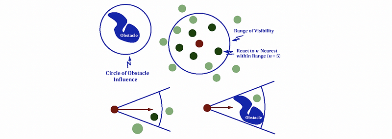
One solution to this is that we strictly restrict the access to information of an agent according to what you think that the agent could reasonably perceive or at least what your gameplay audience has expectations. We can add some constraints on,
- Vision: introduce a distance restriction so that the agent can only see so far
- Field of view: introduce a direction or a forward vector of the agent’s head so that the agent can only view the target it is facing towards
- Single raycast from eyes: the single raycast from the eyes of the agent really enhance the realism of the game
- Consider sounds: the agent can be aware of the audio events generated
- Focus range: the agent can only pay attention to some of the objects in the field of view and then make react to them
- Vague directions for projectiles: if we have some exact projectiles towards the players, the situation can be too challenging for the game players. The negative thing is that it is also quite simple to make some AI helper in your game to make all sorts of things unfair. Probably, we have to make sense to human players by enhancing the Gaussian distribution, and we can also model a reaction time for recognizing.

3. Path Planning
Now, let’s see something about path planning. Path planning is a way we can extend the sort of behavior of our agent. We will still use our steering behaviors, but when we generate a path, the agent will be able to follow.
(1) Graphics
Before we start, let’s review some tools that can be used to facilitate searching. You have to be familiar with the following concepts,
- Graph
- Node
- Edge
- Cost/Weight
If you have any problems with these concepts, you can refer to the following article for more information.
Series: Linear Algebramedium.com
(2) Types of Graphics
The graphics really vary in the challenge we have for that graph. Some of the types are,
- Directed acyclic graph
- Directed cycle graph
- Undirected graph
- Binary tree
- Digraph
(3) Examples of Graphics
- Risk: In the game Risk, we have a graph that is the map for players to move across.

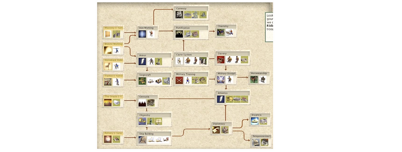
- Civilization: In the Civilization games, we do have a technology tree for interpreting primitive technologies and advanced technologies. This tree is called an RTS dependency tree.
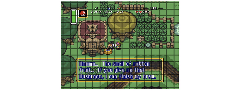
- Zelda: In some of the Zelda games, the graph is in the form of a grid and it is based on sprite tiles.
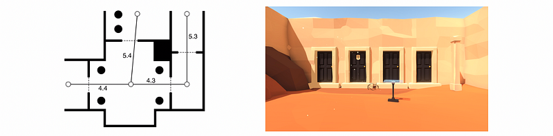
- Door: In the Door game, you have to identify which are the rooms and where are the doorways connecting the rooms. This allows you to place nodes at some coordinate in the game and then define edges based on the room adjacency.
(4) The Definition of Planning
The plan is a series of pre-decisions before we accomplish a goal. We need to have,
- Goal: a goal state
- World: a set of states
- Operators: an operator changes configuration from one state to another state
As it is defined, a plan is a part of the intelligence. So in terms of intelligence planning, we need to have some notion of the current state of the problem, and we need to have some notion of what the state of the problem would look like if we have a solution.
(5) The Definition of Path Planning
Plan planning is one kind of intelligence planning. It has,
- Current State: current location of the agent in the space
- Operators: planned movements of the agent
- World: discretized space such as tiles in a tile-based game, floor locations in 3D, voxels, waypoints, navigation mesh, and so on
- Goal State: move the agent somewhere
(6) Planning Algorithms Metrics
Provided the discretized world and came up with a state representation with that discretized model, you will then apply an algorithm that will search through all the different possibilities of operators being applied to the current state. Then we might go about implementing some algorithm to do this. To find the proper algorithm, we are binding to some metrics,
- Time Complexity: How long does it take to find the answer?
- Space Complexity: How much memory do we need to find the answer?
- Completeness: will it find the answer if there’s only one answer exists?
- Optimizations: will it find the best solution if there’s more than one solution?
(7) Search Strategies
In terms of search strategies, there are two kinds of solutions that we can probably take.
- Blind Search: no assumptions of the graph and no domain knowledge. The only thing we know is the goal state.
- Heuristic Search: there is some domain knowledge (e.g. spatial relationships) that we may leverage by heuristic rules. For video games, there is always some domain knowledge we can get.
(8) Breadth-First Search (BFS)
Breadth-first search (BFS) is an algorithm for searching a tree data structure for a node that satisfies a given property. It starts at the tree root and explores all nodes at the present depth prior to moving on to the nodes at the next depth level. The algorithm should be,
- Expand the root node, search
- Expand all root node’s children, search
- Expand all root node’s grandchildren, search
- Continue
This algorithm is problematic if we have,
- Varying weight edges
- Small memory
Here, you can see the outcome of this algorithm.
(9) Depth-First Search
Depth-first search (DFS) is an algorithm for traversing or searching tree or graph data structures. The algorithm starts at the root node (selecting some arbitrary node as the root node in the case of a graph) and explores as far as possible along each branch before backtracking.
- Expand the root node, search
- Expand the node deepest in the tree, and if there’s no deepest node in the tree, then find the most left one, then search.
- Loop
This algorithm is problematic if we have,
- Requirements for optimizations because we may end up searching the whole tree
- Very silly behavior for an agent. You may find it out from the following outcome because it nearly searched the whole map.

(10) Pathfinding Examples
There are still some problems with pathfinding. Here is a video showing what’s going on in modern games.
(11) Path Planning for Tile-Based Games
Tile-based games are quite common with path planning. These games tend to have discrete locations where there is an agent or an object occupying a cell and then move to another with some atomic discrete movements. You will also occasionally see a tile-based discretized representation where the agents move in a continuous way. So in summary, tile-based games usually have 1-to-1 coordination of path-planning graph and simulation space. And the AIs exist in discrete locations.
(12) Path Planning for Grid Navigation
Commonly, games with grid navigation have 2D tile representations of squares (means 4 to 8 connectivity) or hex (means 6-way connectivity). They often enforce one unit per cell and each cell has a terrain type. We usually don’t have a graph data structure for this type. Instead, we have the grid itself that will implicitly define how we find the path.
(13) Path Planning for Continuous Space
A more complicated situation is that we can hardly do path planning as a graph if we have a continuous space. So we might wish to generate a grid or some other discretized spaces as well. When we do have these issues of generating a discretized space, we have issues of,
- Validity
- Quantization
- Localization
- Agent Movement
- Search Efficiency
(14) Discretization Generation: Grid Lattice
In terms of generating, we need to determine boundaries and terrain type regions, and also these transitions across the terrain. Grid lattice is the common solution and we might have arbitrary polygonal geometry. From that, we need to figure out which cells can we traverse to.
Besides, there are some scenarios we should notice when generating the grids. So we should verify,
- world boundaries don’t go through grid lines
- no obstacle point within a grid cell, or vice versa
- obstacle edges do not intersect grid cell edge

(15) Discretization Generation Issues
- Validity: Suppose A and B are nodes in a discretized space. From any points in node A, can an agent travel in a straight line to any point in adjacent node B? The validity issue really has to do with whether you can move from any point in a discretized area to an adjacent discretized area that is in one of those locations as well.
- Off-Grid: this issue is what to do if an AI entity is off a navigable grid cell? The solution may probably be some random movement and physics engine to slide or bump around and hopefully, this eventually gets to a valid position. Or if the game player isn’t looking, we can just cheat a teleport!
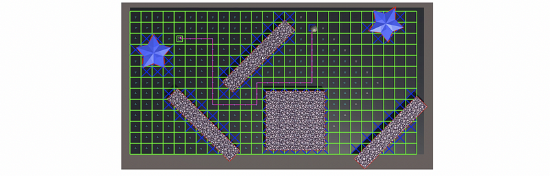
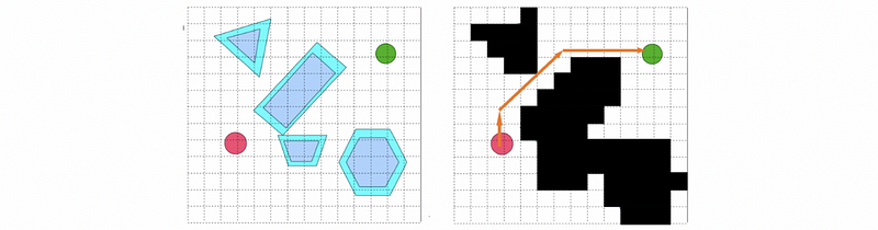
- Continuous Position Vs. Discrete Graph Path: Another issue is the discrete path because of the generated grids. Because the agent follows the discrete pathing plan, it will have awkward and blocky movement which is kind of weird and not natural. Just as the illustration in the following picture, the path we want is actually the green one, however, the one we may finally have is the blue one. However, there are basically two solutions, and we can either do a pre-process or a post-process (aka. string pulling) depending on our perspective.

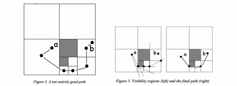
(17) Post Process
The post-process is also called the string-pulling. In the beginning, we may generate some rectangular paths, but then we can clean them up. This method was firstly discussed in the paper Warp Speed: Path Planning for Star Trek®: Armada in 2000. And let’s see figure 3 and figure 5 in this paper for how this works,
(18) Heuristic Greedy Best-First Search
The search efficiency for a grid search is terrible and the search spaces can quickly become huge if we have a bigger map.
So in terms of searches, we might introduce some heuristic (aka. knowledge of the world or some domain knowledge). The easiest way to do that in video games is to consider how close we are to the target. This method is actually called the simple greedy search in which we only expand the nodes that yield the minimum cost. However, there are two issues with this method. First, this algorithm is not complete. Second, greedy means the working solution is not revised, but revisiting the nodes may be beneficial.
Another heuristic is that we can expand nodes closest to the goal first. This is called the heuristic greedy best-first search. In this case, when we hit a dead-end, the algorithm doesn’t give up. Instead, it will backtrack and head down to the actual goal.

Also, from the following outcome, we can tell that this algorithm has a better performance than DFS and BFS.
(19) Dijkstra’s Algorithm
Dijkstra’s algorithm for path searching is actually the weighted-graph version of BFS. It considers the cost of different paths, but BFS simply treats all the edges with the same weight. When all the edges have the same cost, Dijkstra’s algorithm should be exactly the same as BFS. In BFS, we simply have a FIFO model with nodes expanded from left to right in the same layer. However, in Dijkstra’s algorithm, the node with the lowest cost would be expanded first.
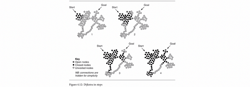
Here, we can find out the outcome of this algorithm is the same as BFS because all the edges have the same cost.
(20) A* Search
A* search is actually a combination of the heuristic greedy best-first search and Dijkstra’s algorithm. For greedy best-first search, we tend to expand the node that is closest to the target first. For Dijkstra’s, we tend to expand the node with the minimum cost. The A* algorithm combines these two approaches for pathfinding.

Here the heuristic part can be any heuristic algorithm. A common heuristic is an Euclidean distance. This is a complete algorithm and it fails only if there’s no solution.
(21) Pathfinding List
In terms of implementing the algorithms, we do need some implementing structures like sorted list, sorted list, priority list, priority queue, or hash table. These are called pathfinding lists. To have the best performance, we have to find a balance between the following four operations of those structures,
- adding an entry to the list
- removing an entry from the list
- finding the smallest element
- finding an entry in the list corresponding to a particular node
Commonly, we can have different types of pathfinding lists and here are some examples of them.
- Linked list: bad efficient because finding may visit all element
- Sorted list: finding is efficient but cost to add increases. This is no good for A* because it adds a lot with relatively fewer find-smallest element calls
- Priority queue/heap: this is an array-based tree structure. Remove the smallest element and add a new element take O(log n).
- Bucketed Priority Queue: this means we have sorted buckets of unsorted lists, and they can be turned for application. This structure is often not worth the trouble.
(22) Problems of A*
It is probably the goal that can not be reached by A*. A possibility is that the agent will search nodes connected to the start node and try to get to the target as close as it can. So the perfect heuristic function that we want for A* should be A* going straight to the correct node in O(p), but this is not possible because such a heuristic solves exactly what we are looking for in the first place. To think about the heuristics, we have to think about some issues like cost.
- Admissible Heuristic: An admissible heuristic is the one that guarantees that the shortest path can be found with the search because it never overestimated the cost of reaching the goal. In short, a heuristic that does not overestimate it is admissible (e.g. Euclidean Distance). In games, it is perfectly acceptable to use either admissible or inadmissible heuristics.
We have the following admissible or inadmissible heuristics for A*,
- Euclidian Distance: admissible
- Cluster Heuristic: may be inadmissible if we need to have the pre-computed distance between cluster
(25) Evaluation of Grid Lattice Navigation
We have discussed lattice navigation and now it’s time to evaluate this method. Some pros are
- Discrete space is uniform and simple
- Usually for games with discrete agent locations but it can be used with continuous coordinates
- Easy to automatically generate
- Good for a large number of units
- A* works well with the grid
But there are also some cons,
- Inefficient use of memory
- The resulting path are jagged/blocky resulting in unnatural movement
- Doesn’t work well to maximize the navigable area
- Search efficiency
- Memory usage
(26) Quadtree
Briefly, we can consider using a quadtree rather than the grid lattice navigation. This is more like a hierarchical grid that we start off with a very large cell, and we check if there are any obstacles within it. Then we subdivide it into four parts for quadtree. Then we just continue that recursively until we figure out a perfect path.

This is a representation of efficient space but it does have some problems.
- This structure is more complicated and parsing
- This structure can result in undesirable quadtree subdivisions if obstacle details don’t line up with quadtree cell boundaries
(27) Path Network
The path network is another structure that does not require the agent to be at one of the path nodes at all times. The agent can be at any point in the terrain allowed by physical simulation. When the agent needs to move to a different location and an obstacle is in the way, the agent can move to the nearest path node accessible by straight-line movement and then find a path through the edges of the path network to another path node near to the desired destination.
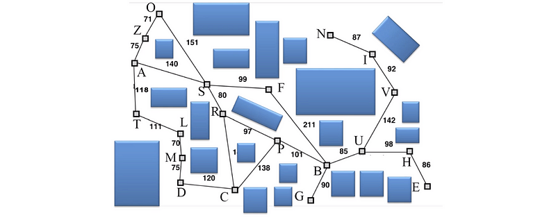
The algorithm of the path network should be as follows,
- Find the closest visible graph node (A)
- Find the closest visible graph node to X (B)
- Search for lowest cost path from A to B
- Move to A
- Traverse path
- Move from B to X
The problem with this structure is that sometimes we may end up in a narrow alley or something else because we can not find a point on the nearby edge. It would be even worse if we can not see a navigation point in the present position. In that situation, what we need to do is to go back and revise the network.
To generate a path network, we can implement some automatic placement. For example, we can,
- Start with seed
- Expand by adding uniformly
- The designer might move, delete, and add manually afterward
- Ensure all the nodes and edges are at least as far from walls as the agent’s collider radius
Another method is called points of visibility (aka. POV) and this means to identify convex angles, and these features create natural inflection points for an efficient path through the environment. The inflection points must be offset by some distance to leave room for the agent. This is one sort of automatic path network and the network is also called the POV graph. This method also has some certain downsides, for example
- it can result in graph bloat
- it can end up going down a rabbit hole of adding more and more software features that never quite work
- it often requires a lot of manual tweaks for offsetting the benefits
(28) Evaluation of Path Network
Aggressive lookahead can result in problems,
- Turns too sharp that causing NPC to slow down
- Overshoot it NPC performance envelope doesn’t match
Also, NPC steering behavior ultimately is not a perfect solution to fixing path network problems. For example,
- Raycasting will still miss some things
- Raycasting can easily become expensive
- Especially problematic on variable height terrain and different terrain types
- NPC make take a shortcut but end up walking in slow terrain instead of staying on the path of fast terrain
So, the path network has some nice benefits like,
- Discretization of space is very small
- Does not require the agent to be at one of the path nodes at all times
- Continuous, non-grid movement in the local area
- Switch between local and remote navigation
- Plays nice with steering behaviors
- Good for FPS and RPGs
- Can indicate special spots (e.g. sniping, crouching, etc.)
But the downsides are,
- Valid NPC positions might not be able to see a node in the network
- Jagged path shape
- Dynamic and rolling terrain issues
- Storage/complexity of network to get good coverage and good path shape
- NPC going off the network path can be dangerous (e.g. getting stuck or so on)
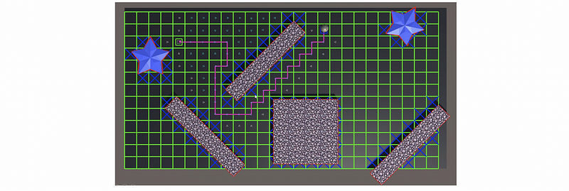
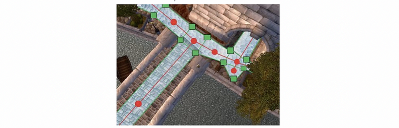
(29) Navigation Mesh (NavMesh)
The navigation mesh defines navigable polygonal areas using convex regions that each has shared adjacent edges that are used to define a graph. So in fact, in the following graph, the blue areas with green edges are the navigation mesh, and the red line denotes the graph which is defined by the navigation mesh. The red line is very much like a path network so it can be searched in that graph. This graph is created by connecting may be the centroid of each of the polygons or in other possibilities, we could use as well. Then across each of these adjacent edges, or we call these the portal edges, is actually the place we can perform an A* search on.
(30) Convexity and Convex Polygon
By definition, convex polygons are polygons that have all internal angles of less than 180 degrees. So all diagonals are contained within the polygon, and a line drawn through a convex polygon in any direction will intersect at exactly two points, and this means that the agent has nothing to collide with.
(33) Greedy Mesh Generation
As far as generating a NavMesh, there is a simple algorithm. So the main thing you need is just a triangulation of the navigable space and you can simply triangulate around from the borders of the space to the edges of the obstacles. So the algorithm is,
- for point A in world points:
- for point B in world points:
- for point C in world points:
- if (it is a valid triangle && !exists):
- add triangle to the mesh
The condition of a valid triangle should be as follows,
- No triangle edge coincident with an obstacle edge unless the same edge
- It can not cross the existing triangle
A greedy version of mesh generation on finding all the triangles is,
- Pick a point on an obstacle or boundary
- Successor points are (1) along the edge of a common obstacle or (2) through world space
- Pick two successor points for the candidate triangle
- see if they are successors of each other
- can not across an existing triangle
- repeat until you can not make more triangles from the original point
- pick a new starting point
So once you have a triangulation, then you can go about merging triangles to make larger regions. There’s no reason to stick with triangles in fact, but if you can make bigger convex regions, you can just attempt to delete an edge between two adjacent triangles and then later on any adjacent convex shapes.
4. Decision Making
(1) Agent’s Behavior
So now the agent is able to move based on our previous discussion. But actually, it should also be able to gather resources, attack, access the computer terminal, open the door, and so on. So the steering behavior blending can sometimes address multiple behaviors but often agents need higher levels of control supported by a decision-making process. For instance, it should be able to avoid steering vectors that negatively interfere, cancel each other out, etc.
(2) The Definition Decision Making
In terms of decision-making, the developers have to determine the recipe for agent pre-planned behaviors. In other words, the programmers should implement the plans. So all the contingencies or exceptional cases anticipated are part of the recipe and if something was missed, the agent is unable to adapt. The decisions are internally made by conditional logic, and they can also include deterministic on non-deterministic conditions.
(3) Types of Decision Making
There are different types of strategies for decision making,
- Reactive decision making: response directly to the environmental state and pre-planned conditional actions
- Deliberative decision making: models discretized environment and interfaces are made to determine the plan that can achieve the goal state
- Reflective decision making: learn from experience
(4) Types of Pre-planned Behaviors
There are several types of pre-planned behaviors as follows,
- Production rules
- Decision trees
- Finite state machine (FSM)
- Behavior trees
And we are going to explain them in the following parts.
(5) Production Rules
The Productions Rules is a simple method for decision making. It actually defines actions to be executed in response to different conditions. So it only has a simple architecture. The problem is that the developers may make some decisions arbitrarily and this makes the project difficult to organize. What’s more, it can also be difficult to understand behavior from looking at the rules. We may also have some situations when rules are ambiguous and conflict. So it makes it kind of a challenge if you want to have your agent perform a sequence of actions, then it requires making a series of rules with stateful triggers.
Here is a quick and dirty example of some production rules,
if (big enemy in sight)
    run away;
if (enemy in sight)
    fight;
if (...)
    ...;
Advanced production rules systems utilize an arbiter that selects from matching rules. A fixed priority arbiter means we will just evaluate the first one that matches from an ordered list for a simple version. We can conduct some priority weighting for rules or sensor events like the firewall rules, or we can simply do some random selection. The production rules can be stateless. An example of random selection with fixed priority is,
if (big enemy in sight && rand() > thresh_1)
    run away;
if (enemy in sight && rand() > thresh_2)
    fight;
if (...)
    ...;
(6) Simple Decision Tree
The decision trees are in some way similar to rule-based systems except for the isolated conditional coupled actions, we now have tree-structured decision logic in terms like a data structure. This is also more readable compared to the rule-based system because we can easily find some dependencies from this tree, so it is really good for simple decision making. However, it can quickly become a mess to manage manually.

(7) Finite State Machine (FSM) Theory
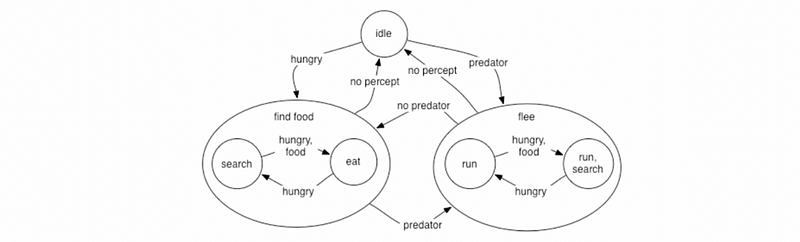
Consider the finite state machine, now we have fairly similar concepts of this kind of conditions on which we act upon. But now, we are going to maintain the stateful information and with a graph structure. So the nodes are the states we have and the edges are transitions. They are directional and the transitions are associated with logic. There are variations where the actions are associated with the transitions but we are not going to mention them in this part. What we are just going to assume is that our states perform an action and continue to perform an action like every time you ask the finite machine to update.
So the model of a finite state machine has the following components,
- a finite number of states S
- an input vocabulary I
- a transition function T(S, I) -> S’
- a start state S₀ ∈ S
- zero or more final states F ⊂ S
The behavior of a finite state machine is that, it
- can only be in one state at a given amount of time
- can make transitions from one state to another to cause an output to take place
- has many states and each of them represents some desired behavior
- can poll the world or respond to events
- can support actions that depend on the state triggering event (Mealy machine)
- can support entry and exit actions associated with states (Moore machine)
The following diagram is a simple example of FSM,

(8) State Machine Problems
There are some problems with the state machines,
- It can be very predictable because we have these specific fixed transactions. This can be solved by using a fuzzy or probabilistic state machine.
- It is also simplistic in what they can do and it can be really hard to scale if we want to have some complicated strategies. But it can be effective by using a hierarchy of FSM stack.
Besides, because the number of states can grow fast because we have an exponential number of events in the world, the FSM can become really huge. So there will be even more problems,
- When it fails, it fails hard. This is because a transition from one state to another requires forethought, and this means we can get stuck in a state or can’t do the correct next action.
- The number of transitions can grow even faster, this means we can not work easily with the sequences of actions
- Memory limitations
(9) Finite State Machine Advantage
However, there are also some benefits of the FSM,
- Ubiquitous: they are popular so we have lots of tools and APIs
- Quick and simple to code: can start from scratch
- Can be easy to debug: because the size is small
- Fast: only have small computational overhead
- Intuitive
- Flexible
- Easy for designers without coding knowledge
(10) Hierarchical Finite State Machine
In terms of some more advanced FSM, one critical model is the hierarchical finite state machine. So if you get to a point that has too many states which can be unmanageable, you may probably need a hierarchical structure. Let’s see an example here,
So this hierarchical FSM is equivalent to regular FSMs, but it adds recursive multi-level evaluations. So is easier for us to think about encapsulation. It seems fairly reasonable if we can maintain a small number of high-level states and then as needed, we can whittle our way down with something specific.
(11) FSM Stack
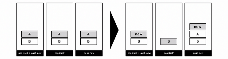
Another approach we can handle the complexity of the FSM is by using a stack. The stack approach allows us to handle the transitions in a slightly different way by pushing onto the stack this new activity. An action is considered complete when it is popped from the stack. So you can pop an activity and then push something new, or you can only pop itself, or if you like, you can just push a new one without popping it out.
There are some dangers of this approach,
- Potential memory leaks: if keep pushing
- May need more restrictions enforced (e.g. we can not have two of the same state on the stack at the same time)
(11) Probabilistic State Machines
Back to the issue of making the agent less predictable, we may consider using a probabilistic state machine.

The basic idea here whenever we have a transition, we are going to couple it with some randomly determined value. We are then going to compare that to a threshold so we might have some basic boolean conditions to decide a transition.

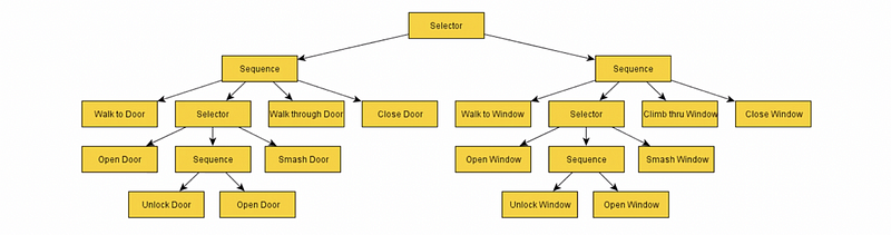
(12) Behavior Trees
Rather than the PSM, the behavior trees are more declarative and generally more understandable. It has some components like,
- Composite
- Decorator
- Leaf: the behaviors

Each component has three return values,
- Success: like true
- Failure: like false
- Running: the behaviors take multiple frames to execute
The behavior trees are still just the reactive planning systems that are very similar to what we have discussed so far for another reactive decision-making. So the tree of behaviors specifies what an agent should do under all circumstances.
The benefit of using the behavior trees is that transitions are decoupled from the states so we have standalone behaviors and we can reuse the tree structure.